A Markovian-based methodology for the life-cycle cost analysis of bridge maintenance interventions under changing deterioration rates

D Fernando1,*, S Walbridge2, B Wan3

1School of Civil Engineering, The University of Queensland, QLD 4072, Australia
2Department of Civil and Environmental Engineering, University of Waterloo, Ontario, N2L 3G1, Canada
3Department of Civil, Construction and Environmental Engineering, Marquette University, Milwaukee, WI 53233, USA

Corresponding author: D Fernando, School of Civil Engineering, the University of Queensland, QLD 4072, Australia, E-mail: dilum. [email protected]

Citation: D Fernando, S Walbridge, B Wan (2020) A Markovian-based methodology for the life-cycle cost analysis of bridge maintenance interventions under changing deterioration rates, J Civil Engg ID 1(1): 1-12.

https://dx.doi.org/10.47890/JCEID/2020/DFernando/12045781

Received Date: : April 28, 2020; Accepted Date: May 04, 2020; Published Date: May 06, 2020

Abstract

Markovian transition probability matrices employing condition states are often used in bridge management systems to determine optimal intervention strategies. This approach assumes a constant deterioration matrix throughout the entire analysis period. In addition, decisions to carry out interventions are normally based on deterioration to predefined condition states, which are generally not linked to structural safety. However, in order to adequately model and evaluate certain intervention options, such as fiber-reinforced polymer (FRP) strengthening, it is necessary to model the impact of the intervention on the deterioration rate, as well as the safety of the structure. This paper presents a Markovian approach to model interventions that impact deteriorating rates. A model employing this approach is proposed, which also accounts for the safety of the structure. A simplified methodology to determine the optimal intervention strategy based on steady state probabilities is also presented. The proposed model and methodology are illustrated in a hypothetical bridge example, where one of the interventions is FRP strengthening of a concrete girder bridge.

Keywords: Changing Deterioration Rates; Markov Chains; Bridge Maintenance Interventions; Optimal Intervention Strategies; Life-cycle Cost Analysis;

Introduction

Bridge managers are required to identify optimal intervention actions to be carried out on bridges so that these structures will continue to provide adequate levels of service to society. In the determination of optimal intervention strategies, bridge managers are often challenged by the variety of different materials that may be used in the interventions, long service lives, and long periods of time between interventions. Existing methodologies [1-4] are sufficient for modeling traditional intervention actions, such as replacement or “patching” of bridge elements, where the intervention can be assumed to change the condition state (CS), but not the deterioration rate. These methodologies are inadequate, however, for evaluating certain intervention actions, which can also influence the deterioration rate of the element.

Walbridge et al. [5] proposed a methodology to evaluate intervention strategies for bridges based on a total life-cycle cost analysis (LCCA), wherein the costs (or impacts) of the various intervention strategies on all of the bridge stakeholders are considered. The proposed methodology used the CS-based Markovian approach to model deterioration, and the costs (or impacts) both during and between the interventions were considered. The methodology was successfully used to evaluate different intervention strategies for a steel roadway bridge. Fernando et al. [6] further extended Walbridge et al.’s [5] methodology to determine the optimal intervention strategy for roadway bridges using steady state probabilities to determine the optimal intervention strategy. Both the Walbridge et al. [5] and Fernando et al. [6] models were limited to interventions where the deterioration matrix remains unchanged, which is a common assumption, made in many existing Markovian-based bridge management systems [7- 9]. In addition, except for the Walbridge et al. [5] model (where the CSs are linked to probabilities of structural failure), it seems that most other CS-based methodologies use predefined CSs, which are not linked to structural failure [7-10], and thus ignore the safety of the structure in the determination of optimal intervention strategy.

Walbridge et al. [5] consider the structural failure of the structure in the CS definition. However, in their analysis, the probability of condition improvement (i.e. replacement of the elements when failed resulting in condition being improved to as new condition) due to structural failure of the elements is ignored.

New intervention possibilities, such as fibre-reinforced polymer (FRP) composite material strengthening, are increasingly being used to retrofit deteriorating reinforced concrete (RC) structures. When a RC beam is strengthened with FRP, the critical deterioration mode of the strengthened beam becomes FRP-toconcrete bond degradation [11-12], which will have a different deterioration rate (more likely a slower deterioration rate) than that of the original RC beam (e.g. due to FRP providing a barrier preventing chloride ingress and reinforcement to reduce rate of fatigue damage, therefore rate of bond degradation becoming faster than the reduced reinforcement corrosion rate). Traditional Markovian models, commonly used in existing bridge management systems, are not capable of modeling changes in the deterioration rate as the result of an intervention. Some efforts have been made [13] to model changing deterioration rates by relaxing the history-independent deterioration assumption commonly used in traditional Markovian-based deterioration models. The most advanced of those models, such as the one described by Robelin and Madanat [13], require considerable computational effort (e.g. to run Monte Carlo simulations) to determine the deterioration matrices. This approach, while attractive when many intervention actions can result in changes of deterioration rates, is computationally demanding when evaluating more simple problems such as interventions on reinforced concrete (RC) structures, where only a few intervention types are being considered. In addition, in the method proposed by Robeling and Madanat [13], structural safety is not explicitly considered.

The current paper presents a methodology to evaluate intervention strategies that result in deterioration rate changes. This methodology employs a modified CS-based transition probability matrix to model deterioration, allowing changes in the deterioration rate to occur during the analysis period as a result of the modeled intervention strategies. A methodology to determine the optimal intervention strategy based on steady state Markovian probabilities is also presented. Finally, the proposed methodology is illustrated using a hypothetical RC bridge girder where one of the considered intervention options is FRP strengthening.

Life-cycle cost (or impact) model

In this section, a new model is proposed by modifying traditional Morkovian deterioration models to account for the changing deterioration rates. This study is specifically motivated by the emergence of new intervention options, such as FRP strengthening, where once strengthened the critical deterioration mechanism may be changed from that of the pre-strengthened element.

For example, a possible intervention for a RC beam is to be strengthened using externally bonded FRP laminates. After such an intervention, the critical deterioration mechanism (in terms of the strength reduction) of the strengthened beam becomes the interfacial damage of the FRP-concrete interface [11-12], which will have a different deterioration rate (typically slower) than that of the original RC beam.

The model developed in this study takes into consideration the following possibilities:

  1. Certain interventions may improve the condition of the element without changing the deterioration rate/mechanism (e.g. paint restoration of a painted steel girder).
  2. Certain types of interventions may improve the condition of the element and also change the deterioration rate/ mechanism (e.g. FRP strengthening of RC girders).
  3. Interventions possible in an intermediate state of deterioration may not be possible if structural failure occurs (e.g. a deteriorating RC beam may be strengthened using FRP strengthening. However, if the beam has experienced structural failure, replacement may be the only viable option). Therefore, it is important to distinguish between the failure CS (typically considered as the worst CS in current practice) and structural failure. Structural failure of an element may occur at any stage irrespective of the CS of the element.
  4. Interventions such as FRP strengthening are aimed predominantly at existing structures. Advantages of FRP strengthening over conventional strengthening methods, e.g. low labor costs, minimal disturbance to the traffic etc., may not have the same significance when used in new structural elements. Therefore, if structural failure occurs in an element (un-strengthened or strengthened), it may or may not be replaced by a new strengthened element. More likely, it will be replaced by a new un-strengthened element.

In the following sections, first a condition-based transition probability matrix considering the structural failure of an element is presented. Secondly, a method to model interventions that will not change the original deterioration rate (explicitly accounting for structural failure)based on steady state Markovian probabilities is presented. Finally, a model is proposed to account for interventions that will result in a change in the deterioration rate.

Condition based transition probability matrix for deterioration modeling

Transition probabilities represent the probability for an element that is in CS i at time period t to be in state j at the following time period (i.e. t+1). A typical transition probability matrix of an element with n CSs can be written as:


P e = p ij e = p 11 e p 12 e p 1n e 0 p 22 e p 2n e 0 0 1                         (1) MathType@MTEF@5@5@+= feaahqart1ev3aqatCvAUfeBSjuyZL2yd9gzLbvyNv2CaerbuLwBLn hiov2DGi1BTfMBaeXatLxBI9gBaerbd9wDYLwzYbItLDharqqtubsr 4rNCHbGeaGqiVu0Je9sqqrpepC0xbbL8F4rqqrFfpeea0xe9Lq=Jc9 vqaqpepm0xbba9pwe9Q8fs0=yqaqpepae9pg0FirpepeKkFr0xfr=x fr=xb9adbiqaceGaciGaaiaabeqaamaabaabaaGcbaGaamiuamaaBa aaleaacaWGLbaabeaakiabg2da9iaadchadaqhaaWcbaGaamyAaiaa dQgaaeaacaWGLbaaaOGaeyypa0ZaamWaaeaafaqabeabeaaaaaqaai aadchadaqhaaWcbaGaaGymaiaaigdaaeaacaWGLbaaaaGcbaGaamiC amaaDaaaleaacaaIXaGaaGOmaaqaaiaadwgaaaaakeaacqWIVlctae aacaWGWbWaa0baaSqaaiaaigdacaWGUbaabaGaamyzaaaaaOqaaiaa icdaaeaacaWGWbWaa0baaSqaaiaaikdacaaIYaaabaGaamyzaaaaaO qaaiabl+UimbqaaiaadchadaqhaaWcbaGaaGOmaiaad6gaaeaacaWG LbaaaaGcbaGaeSO7I0eabaGaeSO7I0eabaGaeSy8I8eabaGaeSO7I0 eabaGaaGimaaqaaiaaicdaaeaacqWIVlctaeaacaaIXaaaaaGaay5w aiaaw2faaiaabccacaqGGaGaaeiiaiaabccacaqGGaGaaeiiaiaabc cacaqGGaGaaeiiaiaabccacaqGGaGaaeiiaiaabccacaqGGaGaaeii aiaabccacaqGGaGaaeiiaiaabccacaqGGaGaaeiiaiaabccacaqGGa GaaeiiaiaabIcacaqGXaGaaeykaaaa@73F1@

with:

j=1 n p ij e =1         i,j p ij e =0 when (i>j)                       (2) MathType@MTEF@5@5@+= feaahqart1ev3aaatCvAUfeBSjuyZL2yd9gzLbvyNv2CaerbuLwBLn hiov2DGi1BTfMBaeXatLxBI9gBaerbd9wDYLwzYbItLDharqqtubsr 4rNCHbGeaGqiVu0Je9sqqrpepC0xbbL8F4rqqrFfpeea0xe9Lq=Jc9 vqaqpepm0xbba9pwe9Q8fs0=yqaqpepae9pg0FirpepeKkFr0xfr=x fr=xb9adbaqaaeGaciGaaiaabeqaamaabaabaaGcbaWaaiqaaeaafa qabeGabaaabaWaaabCaeaacaWGWbWaa0baaSqaaiaadMgacaWGQbaa baGaamyzaaaakiabg2da9iaaigdacaqGGaGaaeiiaiaabccacaqGGa GaaeiiaiaabccacaqGGaGaaeiiaiaabccacqGHaiIicaWGPbGaaiil aiaadQgaaSqaaiaadQgacqGH9aqpcaaIXaaabaGaamOBaaqdcqGHri s5aaGcbaGaamiCamaaDaaaleaacaWGPbGaamOAaaqaaiaadwgaaaGc cqGH9aqpcaaIWaGaaeiiaiaabEhacaqGObGaaeyzaiaab6gacaqGGa GaaiikaiaadMgacqGH+aGpcaWGQbGaaiykaaaaaiaawUhaaiaabcca caqGGaGaaeiiaiaabccacaqGGaGaaeiiaiaabccacaqGGaGaaeiiai aabccacaqGGaGaaeiiaiaabccacaqGGaGaaeiiaiaabccacaqGGaGa aeiiaiaabccacaqGGaGaaeiiaiaabccacaqGOaGaaeOmaiaabMcaaa a@6AD8@

Where index e denotes the element of concern, and n is the number of CSs for element e. An appropriate (stochastic) deterioration model can be used to estimate the transition probabilities in absence of inspection data.

In such a transition matrix the worst (i.e. highest) CS is defined as the CS where the element performance becomes inadequate. However, the probability that the element may experience structural failure within a time interval is not explicitly considered. The probability of the element structural failure is dependent on the current CS of the element. In the current study, a new CS, i.e. CSn+1, is introduced to accommodate the structural failure of the element. The structural failure considered in this study is the result of the applied load exceeding the structural resistance, thus causing a sudden change in the structure condition. Therefore it is assumed that, if the structural failure didn’t occur, deterioration (e.g. corrosion) would continue to follow the normal path as predicted by the stochastic deterioration model. With this assumption, a new transition probability matrix can be written, considering the annual structural failure probability of the element, as:

P ¯ e = p ¯ 11 e p ¯ 12 e p ¯ 1n e p ¯ 1n+1 e 0 p ¯ 22 e p ¯ 2n e p ¯ 2n+1 e 0 0 1 p ¯ nn+1 e p ¯ nn+1 e                           (3) MathType@MTEF@5@5@+= feaahqart1ev3aaatCvAUfeBSjuyZL2yd9gzLbvyNv2CaerbuLwBLn hiov2DGi1BTfMBaeXatLxBI9gBaerbd9wDYLwzYbItLDharqqtubsr 4rNCHbGeaGqiVu0Je9sqqrpepC0xbbL8F4rqqrFfpeea0xe9Lq=Jc9 vqaqpepm0xbba9pwe9Q8fs0=yqaqpepae9pg0FirpepeKkFr0xfr=x fr=xb9adbiqaceGaciGaaiaabeqaamaabaabaaGcbaGabmiuayaara WaaSbaaSqaaiaadwgaaeqaaOGaeyypa0ZaamWaaeaafaqabgabfaaa aaqaaiqadchagaqeamaaDaaaleaacaaIXaGaaGymaaqaaiaadwgaaa aakeaaceWGWbGbaebadaqhaaWcbaGaaGymaiaaikdaaeaacaWGLbaa aaGcbaGaeS47IWeabaGabmiCayaaraWaa0baaSqaaiaaigdacaWGUb aabaGaamyzaaaaaOqaaiqadchagaqeamaaDaaaleaacaaIXaGaamOB aiabgUcaRiaaigdaaeaacaWGLbaaaaGcbaGaaGimaaqaaiqadchaga qeamaaDaaaleaacaaIYaGaaGOmaaqaaiaadwgaaaaakeaacqWIVlct aeaaceWGWbGbaebadaqhaaWcbaGaaGOmaiaad6gaaeaacaWGLbaaaa GcbaGabmiCayaaraWaa0baaSqaaiaaikdacaWGUbGaey4kaSIaaGym aaqaaiaadwgaaaaakeaacqWIUlstaeaacqWIUlstaeaacqWIXlYtae aacqWIUlstaeaacqWIUlstaeaacaaIWaaabaGaaGimaaqaaiabl+Ui mbqaaiaaigdacqGHsislceWGWbGbaebadaqhaaWcbaGaamOBaiaad6 gacqGHRaWkcaaIXaaabaGaamyzaaaaaOqaaiqadchagaqeamaaDaaa leaacaWGUbGaamOBaiabgUcaRiaaigdaaeaacaWGLbaaaaaaaOGaay 5waiaaw2faaiaabccacaqGGaGaaeiiaiaabccacaqGGaGaaeiiaiaa bccacaqGGaGaaeiiaiaabccacaqGGaGaaeiiaiaabccacaqGGaGaae iiaiaabccacaqGGaGaaeiiaiaabccacaqGGaGaaeiiaiaabccacaqG GaGaaeiiaiaabccacaqGGaGaaeikaiaabodacaqGPaaaaa@8A84@

Where

p ¯ ij e = 1 F i e p ij e       j<n+1   j=1 n p ¯ ij e =1 F i e          i,j p ¯ in+1 e = F i e        p ¯ ij e =0 when (i>j)                          (4) MathType@MTEF@5@5@+= feaahqart1ev3aaatCvAUfeBSjuyZL2yd9gzLbvyNv2CaerbuLwBLn hiov2DGi1BTfMBaeXatLxBI9gBaerbd9wDYLwzYbItLDharqqtubsr 4rNCHbGeaGqiVu0Je9sqqrpepC0xbbL8F4rqqrFfpeea0xe9Lq=Jc9 vqaqpepm0xbba9pwe9Q8fs0=yqaqpepae9pg0FirpepeKkFr0xfr=x fr=xb9adbaqaaeGaciGaaiaabeqaamaabaabaaGcbaWaaiqaaqaabe qaaiqadchagaqeamaaDaaaleaacaWGPbGaamOAaaqaaiaadwgaaaGc cqGH9aqpdaqadaqaaiaaigdacqGHsislcaWGgbWaa0baaSqaaiaadM gaaeaacaWGLbaaaaGccaGLOaGaayzkaaGaamiCamaaDaaaleaacaWG PbGaamOAaaqaaiaadwgaaaGccaqGGaGaaeiiaiaabccacaqGGaGaae iiaiaabccacqGHaiIicaWGQbGaeyipaWJaamOBaiabgUcaRiaaigda caqGGaGaaeiiaaqaamaaqahabaGabmiCayaaraWaa0baaSqaaiaadM gacaWGQbaabaGaamyzaaaakiabg2da9iaaigdacqGHsislcaWGgbWa a0baaSqaaiaadMgaaeaacaWGLbaaaOGaaeiiaiaabccacaqGGaGaae iiaiaabccacaqGGaGaaeiiaiaabccacaqGGaGaeyiaIiIaamyAaiaa cYcacaWGQbaaleaacaWGQbGaeyypa0JaaGymaaqaaiaad6gaa0Gaey yeIuoaaOqaaiqadchagaqeamaaDaaaleaacaWGPbGaamOBaiabgUca RiaaigdaaeaacaWGLbaaaOGaeyypa0JaamOramaaDaaaleaacaWGPb aabaGaamyzaaaakiaabccacaqGGaGaaeiiaiaabccacaqGGaGaaeii aaqaaiqadchagaqeamaaDaaaleaacaWGPbGaamOAaaqaaiaadwgaaa GccqGH9aqpcaaIWaGaaeiiaiaabEhacaqGObGaaeyzaiaab6gacaqG GaGaaiikaiaadMgacqGH+aGpcaWGQbGaaiykaaaacaGL7baacaqGGa GaaeiiaiaabccacaqGGaGaaeiiaiaabccacaqGGaGaaeiiaiaabcca caqGGaGaaeiiaiaabccacaqGGaGaaeiiaiaabccacaqGGaGaaeiiai aabccacaqGGaGaaeiiaiaabccacaqGGaGaaeiiaiaabccacaqGGaGa aeikaiaabsdacaqGPaaaaa@978E@

Where Fei is the structural failure probability of an element in CS i.

Case 1: When the interventions result in elements with properties that are similar to the original elements

In typical Markovian models, interventions are assumed to improve the condition of the elements, but assumed not to change the deterioration rate. Therefore, deterioration matrix remains the same after the interventions. If the element undergoes structural failure, and is replaced by an element similar to the original, then again the deterioration rate can be assumed to remain unchanged.

The effectiveness matrix of the intervention carried out at CSs 1, 2, …, n+1can be defined using the transition probabilities representing the probability for an element that is in CS i at the time of intervention to be in state j after the interventions set x as:


R e x, i ' = r ij e,x = r 1,1 e,x r 1,2 e,x r 1,n e,x r 2,1 e,x r 2,2 e,x r 2,n e,x r n+1,1 e,x r n+1,2 e,x r n+1,n e,x                       (5) MathType@MTEF@5@5@+= feaahqart1ev3aqatCvAUfeBSjuyZL2yd9gzLbvyNv2CaerbuLwBLn hiov2DGi1BTfMBaeXatLxBI9gBaerbd9wDYLwzYbItLDharqqtubsr 4rNCHbGeaGqiVu0Je9sqqrpepC0xbbL8F4rqqrFfpeea0xe9Lq=Jc9 vqaqpepm0xbba9pwe9Q8fs0=yqaqpepae9pg0FirpepeKkFr0xfr=x fr=xb9adbiqaceGaciGaaiaabeqaamaabaabaaGcbaGaamOuamaaBa aaleaacaWGLbaabeaakmaabmaabaGaamiEaiaacYcacaWGPbWaaWba aSqabeaacaGGNaaaaaGccaGLOaGaayzkaaGaeyypa0JaamOCamaaDa aaleaacaWGPbGaamOAaaqaaiaadwgacaGGSaGaamiEaaaakiabg2da 9maadmaabaqbaeqabqabaaaaaeaacaWGYbWaa0baaSqaaiaaigdaca GGSaGaaGymaaqaaiaadwgacaGGSaGaamiEaaaaaOqaaiaadkhadaqh aaWcbaGaaGymaiaacYcacaaIYaaabaGaamyzaiaacYcacaWG4baaaa GcbaGaeS47IWeabaGaamOCamaaDaaaleaacaaIXaGaaiilaiaad6ga aeaacaWGLbGaaiilaiaadIhaaaaakeaacaWGYbWaa0baaSqaaiaaik dacaGGSaGaaGymaaqaaiaadwgacaGGSaGaamiEaaaaaOqaaiaadkha daqhaaWcbaGaaGOmaiaacYcacaaIYaaabaGaamyzaiaacYcacaWG4b aaaaGcbaGaeS47IWeabaGaamOCamaaDaaaleaacaaIYaGaaiilaiaa d6gaaeaacaWGLbGaaiilaiaadIhaaaaakeaacqWIUlstaeaacqWIUl staeaacqWIXlYtaeaacqWIUlstaeaacaWGYbWaa0baaSqaaiaad6ga cqGHRaWkcaaIXaGaaiilaiaaigdaaeaacaWGLbGaaiilaiaadIhaaa aakeaacaWGYbWaa0baaSqaaiaad6gacqGHRaWkcaaIXaGaaiilaiaa ikdaaeaacaWGLbGaaiilaiaadIhaaaaakeaacqWIVlctaeaacaWGYb Waa0baaSqaaiaad6gacqGHRaWkcaaIXaGaaiilaiaad6gaaeaacaWG LbGaaiilaiaadIhaaaaaaaGccaGLBbGaayzxaaGaaeiiaiaabccaca qGGaGaaeiiaiaabccacaqGGaGaaeiiaiaabccacaqGGaGaaeiiaiaa bccacaqGGaGaaeiiaiaabccacaqGGaGaaeiiaiaabccacaqGGaGaae iiaiaabccacaqGGaGaaeiiaiaabIcacaqG1aGaaeykaaaa@9FBD@

With the properties:

r ij e,x 0      i,j j=1 n r ij e,x =1  i= i ' j=1 n r ij e,x =0  i i '                      (6) MathType@MTEF@5@5@+= feaahqart1ev3aaatCvAUfeBSjuyZL2yd9gzLbvyNv2CaerbuLwBLn hiov2DGi1BTfMBaeXatLxBI9gBaerbd9wDYLwzYbItLDharqqtubsr 4rNCHbGeaGqiVu0Je9sqqrpepC0xbbL8F4rqqrFfpeea0xe9Lq=Jc9 vqaqpepm0xbba9pwe9Q8fs0=yqaqpepae9pg0FirpepeKkFr0xfr=x fr=xb9adbaqaaeGaciGaaiaabeqaamaabaabaaGcbaWaaiqaaqaabe qaaiaadkhadaqhaaWcbaGaamyAaiaadQgaaeaacaWGLbGaaiilaiaa dIhaaaGccqGHLjYScaaIWaGaaeiiaiaabccacaqGGaGaaeiiaiaabc cacaqGGaGaeyiaIiIaamyAaiaacYcacaWGQbaabaWaaabCaeaacaWG YbWaa0baaSqaaiaadMgacaWGQbaabaGaamyzaiaacYcacaWG4baaaO Gaeyypa0JaaGymaiaabccacaqGGaGaeyiaIiIaamyAaiabg2da9iaa dMgadaahaaWcbeqaaiaacEcaaaaabaGaamOAaiabg2da9iaaigdaae aacaWGUbaaniabggHiLdaakeaadaaeWbqaaiaadkhadaqhaaWcbaGa amyAaiaadQgaaeaacaWGLbGaaiilaiaadIhaaaGccqGH9aqpcaaIWa GaaeiiaiaabccacqGHaiIicaWGPbGaeyiyIKRaamyAamaaCaaaleqa baGaai4jaaaaaeaacaWGQbGaeyypa0JaaGymaaqaaiaad6gaa0Gaey yeIuoaaaGccaGL7baacaqGGaGaaeiiaiaabccacaqGGaGaaeiiaiaa bccacaqGGaGaaeiiaiaabccacaqGGaGaaeiiaiaabccacaqGGaGaae iiaiaabccacaqGGaGaaeiiaiaabccacaqGGaGaaeiiaiaabccacaqG OaGaaeOnaiaabMcaaaa@7CC3@

Where ' i denotes the CSs where interventions will be carried out. Note that this is an n+1 by n matrix, as any intervention carried out on the element will improve the condition, thus the probability of structural failure is assumed to be negligible immediately after the intervention. Also, it is reasonable to assume that the interventions on any of the CSs i’=1, 2, ...,n (i.e. non-structural failure CSs) will be carried out only if the element does not experience structural failure prior to the intervention. If the element experience structural failure, it will be immediately replaced by a new element. Therefore the resulting deterioration-intervention matrix for a single time interval can be written as:


Q ¯ e x, i ' = q ¯ ij e = p ^ ij e + 1 p ¯ in+1 e r ij e,x + p ¯ in+1 e r n+1j e,x i,j=1,2,...,n              (7) MathType@MTEF@5@5@+= feaahqart1ev3aaatCvAUfeBSjuyZL2yd9gzLbvyNv2CaerbuLwBLn hiov2DGi1BTfMBaeXatLxBI9gBaerbd9wDYLwzYbItLDharqqtubsr 4rNCHbGeaGqiVu0Je9sqqrpepC0xbbL8F4rqqrFfpeea0xe9Lq=Jc9 vqaqpepm0xbba9pwe9Q8fs0=yqaqpepae9pg0FirpepeKkFr0xfr=x fr=xb9adbiqaceGaciGaaiaabeqaamaabaabaaGcbaGabmyuayaara WaaSbaaSqaaiaadwgaaeqaaOWaaeWaaeaacaWG4bGaaiilaiaadMga daahaaWcbeqaaiaacEcaaaaakiaawIcacaGLPaaacqGH9aqpceWGXb GbaebadaqhaaWcbaGaamyAaiaadQgaaeaacaWGLbaaaOGaeyypa0Ja bmiCayaajaWaa0baaSqaaiaadMgacaWGQbaabaGaamyzaaaakiabgU caRmaadmaabaGaaGymaiabgkHiTiqadchagaqeamaaDaaaleaacaWG PbGaamOBaiabgUcaRiaaigdaaeaacaWGLbaaaaGccaGLBbGaayzxaa GaamOCamaaDaaaleaacaWGPbGaamOAaaqaaiaadwgacaGGSaGaamiE aaaakiabgUcaRiqadchagaqeamaaDaaaleaacaWGPbGaamOBaiabgU caRiaaigdaaeaacaWGLbaaaOGaamOCamaaDaaaleaacaWGUbGaey4k aSIaaGymaiaadQgaaeaacaWGLbGaaiilaiaadIhaaaGcdaqfqaqabS qaaaqab0qaaaaakiaadMgacaGGSaGaamOAaiabg2da9iaaigdacaGG SaGaaGOmaiaacYcacaGGUaGaaiOlaiaac6cacaGGSaGaaiOBaiaabc cacaqGGaGaaeiiaiaabccacaqGGaGaaeiiaiaabccacaqGGaGaaeii aiaabccacaqGGaGaaeiiaiaabccacaqGGaGaaeikaiaabEdacaqGPa aaaa@7A2F@

Where


p ^ ij e = p ¯ ij e      i i ' p ^ ij e =0     i= i '                 (8) MathType@MTEF@5@5@+= feaahqart1ev3aaatCvAUfeBSjuyZL2yd9gzLbvyNv2CaerbuLwBLn hiov2DGi1BTfMBaeXatLxBI9gBaerbd9wDYLwzYbItLDharqqtubsr 4rNCHbGeaGqiVu0Je9sqqrpepC0xbbL8F4rqqrFfpeea0xe9Lq=Jc9 vqaqpepm0xbba9pwe9Q8fs0=yqaqpepae9pg0FirpepeKkFr0xfr=x fr=xb9adbaqaaeGaciGaaiaabeqaamaabaabaaGcbaWaaiqaaqaabe qaaiqadchagaqcamaaDaaaleaacaWGPbGaamOAaaqaaiaadwgaaaGc cqGH9aqpceWGWbGbaebadaqhaaWcbaGaamyAaiaadQgaaeaacaWGLb aaaOGaaeiiaiaabccacaqGGaGaaeiiaiaabccacqGHaiIicaWGPbGa eyiyIKRaamyAamaaCaaaleqabaGaai4jaaaaaOqaaiqadchagaqcam aaDaaaleaacaWGPbGaamOAaaqaaiaadwgaaaGccqGH9aqpcaaIWaGa aeiiaiaabccacaqGGaGaaeiiamaaxababaaaleaaaeqaaOGaeyiaIi IaamyAaiabg2da9iaadMgadaahaaWcbeqaaiaacEcaaaaaaOGaay5E aaGaaeiiaiaabccacaqGGaGaaeiiaiaabccacaqGGaGaaeiiaiaabc cacaqGGaGaaeiiaiaabccacaqGGaGaaeiiaiaabccacaqGGaGaaeii aiaabIcacaqG4aGaaeykaaaa@6214@

The CS of the element in any given year can be obtained by multiplying the CS of the element at the beginning of each year by deterioration-intervention matrix, ( ) ' Q x,i e , i.e.:

Π e t,x, i ' = Π e 0 Q ¯ e x, i i t                  (9) MathType@MTEF@5@5@+= feaahqart1ev3aaatCvAUfeBSjuyZL2yd9gzLbvyNv2CaerbuLwBLn hiov2DGi1BTfMBaeXatLxBI9gBaerbd9wDYLwzYbItLDharqqtubsr 4rNCHbGeaGqiVu0Je9sqqrpepC0xbbL8F4rqqrFfpeea0xe9Lq=Jc9 vqaqpepm0xbba9pwe9Q8fs0=yqaqpepae9pg0FirpepeKkFr0xfr=x fr=xb9adbiqaceGaciGaaiaabeqaamaabaabaaGcbaGaeuiOda1aaS baaSqaaiaadwgaaeqaaOWaaeWaaeaacaWG0bGaaiilaiaadIhacaGG SaGaamyAamaaCaaaleqabaGaai4jaaaaaOGaayjkaiaawMcaaiabg2 da9iabfc6aqnaaBaaaleaacaWGLbaabeaakmaabmaabaGaaGimaaGa ayjkaiaawMcaamaabmaabaGabmyuayaaraWaa0baaSqaaiaadwgaae aaaaGcdaqadaqaaiaadIhacaGGSaGaamyAamaaCaaaleqabaGaamyA aaaaaOGaayjkaiaawMcaaaGaayjkaiaawMcaamaaCaaaleqabaGaam iDaaaakiaabccacaqGGaGaaeiiaiaabccacaqGGaGaaeiiaiaabcca caqGGaGaaeiiaiaabccacaqGGaGaaeiiaiaabccacaqGGaGaaeiiai aabccacaqGGaGaaeikaiaabMdacaqGPaaaaa@5C22@

where

Π e 0 = π 1 e 0 π 2 e 0 π n e 0 MathType@MTEF@5@5@+= feaahqart1ev3aaatCvAUfeBSjuyZL2yd9gzLbvyNv2CaerbuLwBLn hiov2DGi1BTfMBaeXatLxBI9gBaerbd9wDYLwzYbItLDharqqtubsr 4rNCHbGeaGqiVu0Je9sqqrpepC0xbbL8F4rqqrFfpeea0xe9Lq=Jc9 vqaqpepm0xbba9pwe9Q8fs0=yqaqpepae9pg0FirpepeKkFr0xfr=x fr=xb9adbiqaceGaciGaaiaabeqaamaabaabaaGcbaGaeuiOda1aaS baaSqaaiaadwgaaeqaaOWaaeWaaeaacaaIWaaacaGLOaGaayzkaaGa eyypa0ZaaiWaaeaafaqabeqaeaaaaeaacqaHapaCdaqhaaWcbaGaaG ymaaqaaiaadwgaaaGcdaqadaqaaiaaicdaaiaawIcacaGLPaaaaeaa cqaHapaCdaqhaaWcbaGaaGOmaaqaaiaadwgaaaGcdaqadaqaaiaaic daaiaawIcacaGLPaaaaeaacqWIVlctaeaacqaHapaCdaqhaaWcbaGa amOBaaqaaiaadwgaaaGcdaqadaqaaiaaicdaaiaawIcacaGLPaaaaa aacaGL7bGaayzFaaaaaa@51DB@

is the CS distribution of the element at time t=0.

The expected total costs or impacts in any given year are the sum of intervention costs (in both structural failure and non-structural failure CSs) and costs incurred due to the normal operations of the bridge. Therefore, the expected cost or value of impacts in any given year can be written as:


E V t x, i ' = i= i ' j=1 n π j e t1 p ¯ ji e a=1 A c a,x e,I                         + j=1 n π j e t1 p ¯ jn+1 e a=1 A c a e,f + j=1 n π j e t a=1 A c a,j e,D 1 d t x, i ' d T,t                         (10) MathType@MTEF@5@5@+= feaahqart1ev3aaatCvAUfeBSjuyZL2yd9gzLbvyNv2CaerbuLwBLn hiov2DGi1BTfMBaeXatLxBI9gBaerbd9wDYLwzYbItLDharqqtubsr 4rNCHbGeaGqiVu0Je9sqqrpepC0xbbL8F4rqqrFfpeea0xe9Lq=Jc9 vqaqpepm0xbba9pwe9Q8fs0=yqaqpepae9pg0FirpepeKkFr0xfr=x fr=xb9adbiqaceGaciGaaiaabeqaamaabaabaaGceaqabeaacaWGfb WaaeWaaeaacaWGwbWaaSbaaSqaaiaadshaaeqaaOWaaeWaaeaacaWG 4bGaaiilaiaadMgadaahaaWcbeqaaiaacEcaaaaakiaawIcacaGLPa aaaiaawIcacaGLPaaacqGH9aqpdaaeWbqaamaaqahabaGaeqiWda3a a0baaSqaaiaadQgaaeaacaWGLbaaaOWaaeWaaeaacaWG0bGaeyOeI0 IaaGymaaGaayjkaiaawMcaaiqadchagaqeamaaDaaaleaacaWGQbGa amyAaaqaaiaadwgaaaGcdaaeWbqaaiaadogadaqhaaWcbaGaamyyai aacYcacaWG4baabaGaamyzaiaacYcacaWGjbaaaaqaaiaadggacqGH 9aqpcaaIXaaabaGaamyqaaqdcqGHris5aaWcbaGaamOAaiabg2da9i aaigdaaeaacaWGUbaaniabggHiLdaaleaacqGHaiIicaWGPbGaeyyp a0JaamyAamaaCaaameqabaGaai4jaaaaaSqaaaqdcqGHris5aaGcba GaaeiiaiaabccacaqGGaGaaeiiaiaabccacaqGGaGaaeiiaiaabcca caqGGaGaaeiiaiaabccacaqGGaGaaeiiaiaabccacaqGGaGaaeiiai aabccacaqGGaGaaeiiaiaabccacaqGGaGaaeiiaiaabccacaqGGaGa ey4kaSYaaabCaeaacqaHapaCdaqhaaWcbaGaamOAaaqaaiaadwgaaa GcdaqadaqaaiaadshacqGHsislcaaIXaaacaGLOaGaayzkaaGabmiC ayaaraWaa0baaSqaaiaadQgacaWGUbGaey4kaSIaaGymaaqaaiaadw gaaaaabaGaamOAaiabg2da9iaaigdaaeaacaWGUbaaniabggHiLdGc daaeWbqaaiaadogadaqhaaWcbaGaamyyaaqaaiaadwgacaGGSaGaam OzaaaaaeaacaWGHbGaeyypa0JaaGymaaqaaiaadgeaa0GaeyyeIuoa kiabgUcaRmaaqahabaGaeqiWda3aa0baaSqaaiaadQgaaeaacaWGLb aaaOWaaeWaaeaacaWG0baacaGLOaGaayzkaaWaaabCaeaacaWGJbWa a0baaSqaaiaadggacaGGSaGaamOAaaqaaiaadwgacaGGSaGaamiraa aaaeaacaWGHbGaeyypa0JaaGymaaqaaiaadgeaa0GaeyyeIuoaaSqa aiaadQgacqGH9aqpcaaIXaaabaGaamOBaaqdcqGHris5aOWaaeWaae aacaaIXaGaeyOeI0YaaSaaaeaacaWGKbWaaSbaaSqaaiaadshaaeqa aOWaaeWaaeaacaWG4bGaaiilaiaadMgadaahaaWcbeqaaiaacEcaaa aakiaawIcacaGLPaaaaeaacaWGKbWaaSbaaSqaaiaadsfacaGGSaGa amiDaaqabaaaaaGccaGLOaGaayzkaaGaaeiiaiaabccacaqGGaGaae iiaiaabccacaqGGaGaaeiiaiaabccacaqGGaGaaeiiaiaabccacaqG GaGaaeiiaiaabccacaqGGaGaaeiiaiaabccacaqGGaGaaeiiaiaabc cacaqGGaGaaeiiaiaabccacaqGGaGaaeikaiaabgdacaqGWaGaaeyk aaaaaa@CB81@

where ( 1) πej(t −1) is the probability of element being in CS j in time t-1, c e,Ia,xis the value of impact a in carrying out intervention x in non-structural failure CS ' i on element e, c e,fais the value of impact a in an event of the failure of element e, ce,D a,jis the value of impact a when the element is in operation and in CS j, d T ,tis the length of the time interval t in days, and ' dt (x,i) is the number of days per time interval t that the structure is out of service due to interventions x, which can be calculated as:


d t x, i ' = i= i ' j=1 n π j e t1 p ¯ ji e d x e,I + j=1 n π j e t1 p ¯ jn+1 e d n+1 e,f                (11) MathType@MTEF@5@5@+= feaahqart1ev3aqatCvAUfeBSjuyZL2yd9gzLbvyNv2CaerbuLwBLn hiov2DGi1BTfMBaeXatLxBI9gBaerbd9wDYLwzYbItLDharqqtubsr 4rNCHbGeaGqiVu0Je9sqqrpepC0xbbL8F4rqqrFfpeea0xe9Lq=Jc9 vqaqpepm0xbba9pwe9Q8fs0=yqaqpepae9pg0FirpepeKkFr0xfr=x fr=xb9adbiqaceGaciGaaiaabeqaamaabaabaaGcbaGaamizamaaBa aaleaacaWG0baabeaakmaabmaabaGaamiEaiaacYcacaWGPbWaaWba aSqabeaacaGGNaaaaaGccaGLOaGaayzkaaGaeyypa0ZaaabCaeaada aeWbqaaiabec8aWnaaDaaaleaacaWGQbaabaGaamyzaaaakmaabmaa baGaamiDaiabgkHiTiaaigdaaiaawIcacaGLPaaaceWGWbGbaebada qhaaWcbaGaamOAaiaadMgaaeaacaWGLbaaaOGaamizamaaDaaaleaa caWG4baabaGaamyzaiaacYcacaWGjbaaaaqaaiaadQgacqGH9aqpca aIXaaabaGaamOBaaqdcqGHris5aaWcbaGaeyiaIiIaamyAaiabg2da 9iaadMgadaahaaadbeqaaiaacEcaaaaaleaaa0GaeyyeIuoakiabgU caRmaaqahabaGaeqiWda3aa0baaSqaaiaadQgaaeaacaWGLbaaaOWa aeWaaeaacaWG0bGaeyOeI0IaaGymaaGaayjkaiaawMcaaiqadchaga qeamaaDaaaleaacaWGQbGaamOBaiabgUcaRiaaigdaaeaacaWGLbaa aaqaaiaadQgacqGH9aqpcaaIXaaabaGaamOBaaqdcqGHris5aOGaam izamaaDaaaleaacaWGUbGaey4kaSIaaGymaaqaaiaadwgacaGGSaGa amOzaaaakiaabccacaqGGaGaaeiiaiaabccacaqGGaGaaeiiaiaabc cacaqGGaGaaeiiaiaabccacaqGGaGaaeiiaiaabccacaqGGaGaaeii aiaabIcacaqGXaGaaeymaiaabMcaaaa@8236@

Where d e,Ixis the number of days when the element will be out of service for interventions x carried out on non-structural failure CSs ' i , and de,f n+1 is the number of days when the element will be out of service due to failure. The optimal intervention strategy, i.e. intervention set x, and CSs ' i where the interventions will be carried out can be written as:


xX, i ' i,E T V t x, i ' =min t=0 T E V t x, i ' 1 1+r t                   (12) MathType@MTEF@5@5@+= feaahqart1ev3aaatCvAUfeBSjuyZL2yd9gzLbvyNv2CaerbuLwBLn hiov2DGi1BTfMBaeXatLxBI9gBaerbd9wDYLwzYbItLDharqqtubsr 4rNCHbGeaGqiVu0Je9sqqrpepC0xbbL8F4rqqrFfpeea0xe9Lq=Jc9 vqaqpepm0xbba9pwe9Q8fs0=yqaqpepae9pg0FirpepeKkFr0xfr=x fr=xb9adbiqaceGaciGaaiaabeqaamaabaabaaGcbaGaeyiaIiIaam iEaiabgIGiolaadIfacaGGSaGaamyAamaaCaaaleqabaGaai4jaaaa kiabgIGiolaadMgacaGGSaGaamyramaabmaabaGaamivaiaadAfada WgaaWcbaGaamiDaaqabaGcdaqadaqaaiaadIhacaGGSaGaamyAamaa CaaaleqabaGaai4jaaaaaOGaayjkaiaawMcaaaGaayjkaiaawMcaai abg2da9iGac2gacaGGPbGaaiOBamaadmaabaWaaabCaeaacaWGfbWa aeWaaeaacaWGwbWaaSbaaSqaaiaadshaaeqaaOWaaeWaaeaacaWG4b GaaiilaiaadMgadaahaaWcbeqaaiaacEcaaaaakiaawIcacaGLPaaa aiaawIcacaGLPaaadaqadaqaamaalaaabaGaaGymaaqaaiaaigdacq GHRaWkcaWGYbaaaaGaayjkaiaawMcaamaaCaaaleqabaGaamiDaaaa aeaacaWG0bGaeyypa0JaaGimaaqaaiaadsfaa0GaeyyeIuoaaOGaay 5waiaaw2faaiaabccacaqGGaGaaeiiaiaabccacaqGGaGaaeiiaiaa bccacaqGGaGaaeiiaiaabccacaqGGaGaaeiiaiaabccacaqGGaGaae iiaiaabccacaqGGaGaaeiiaiaabIcacaqGXaGaaeOmaiaabMcaaaa@7347@

Case 2: When the interventions use elements with different properties from the original elements

When an intervention changes the deterioration rate, the above described modeling approach is no longer applicable. If the deterioration rate changes, a new deterioration matrix is needed to model for the post-intervention element. If such an intervention of the original element is carried out in CSi, we can assume that the element CS will transit to a new deterioration matrix, which has the transition probabilities corresponding to the new element (postintervention element) deterioration rate. In order to represent this in a transition probability matrix, the deterioration of the new element (denote by index 2) is modeled using k+1 CSs with CS k+1 representing the structural failure of the new element:


P ¯ 2 = p ¯ 11 2 p ¯ 12 2 p ¯ 1k 2 p ¯ 1k+1 2 0 p ¯ 22 2 p ¯ 2k 2 p ¯ 2k+1 2 0 0 1 p ¯ kk+1 2 p ¯ kk+1 2                           (13) MathType@MTEF@5@5@+= feaahqart1ev3aaatCvAUfeBSjuyZL2yd9gzLbvyNv2CaerbuLwBLn hiov2DGi1BTfMBaeXatLxBI9gBaerbd9wDYLwzYbItLDharqqtubsr 4rNCHbGeaGqiVu0Je9sqqrpepC0xbbL8F4rqqrFfpeea0xe9Lq=Jc9 vqaqpepm0xbba9pwe9Q8fs0=yqaqpepae9pg0FirpepeKkFr0xfr=x fr=xb9adbiqaceGaciGaaiaabeqaamaabaabaaGcbaGabmiuayaara WaaSbaaSqaaiaaikdaaeqaaOGaeyypa0ZaamWaaeaafaqabgabfaaa aaqaaiqadchagaqeamaaDaaaleaacaaIXaGaaGymaaqaaiaaikdaaa aakeaaceWGWbGbaebadaqhaaWcbaGaaGymaiaaikdaaeaacaaIYaaa aaGcbaGaeS47IWeabaGabmiCayaaraWaa0baaSqaaiaaigdacaWGRb aabaGaaGOmaaaaaOqaaiqadchagaqeamaaDaaaleaacaaIXaGaam4A aiabgUcaRiaaigdaaeaacaaIYaaaaaGcbaGaaGimaaqaaiqadchaga qeamaaDaaaleaacaaIYaGaaGOmaaqaaiaaikdaaaaakeaacqWIVlct aeaaceWGWbGbaebadaqhaaWcbaGaaGOmaiaadUgaaeaacaaIYaaaaa GcbaGabmiCayaaraWaa0baaSqaaiaaikdacaWGRbGaey4kaSIaaGym aaqaaiaaikdaaaaakeaacqWIUlstaeaacqWIUlstaeaacqWIXlYtae aacqWIUlstaeaacqWIUlstaeaacaaIWaaabaGaaGimaaqaaiabl+Ui mbqaaiaaigdacqGHsislceWGWbGbaebadaqhaaWcbaGaam4AaiaadU gacqGHRaWkcaaIXaaabaGaaGOmaaaaaOqaaiqadchagaqeamaaDaaa leaacaWGRbGaam4AaiabgUcaRiaaigdaaeaacaaIYaaaaaaaaOGaay 5waiaaw2faaiaabccacaqGGaGaaeiiaiaabccacaqGGaGaaeiiaiaa bccacaqGGaGaaeiiaiaabccacaqGGaGaaeiiaiaabccacaqGGaGaae iiaiaabccacaqGGaGaaeiiaiaabccacaqGGaGaaeiiaiaabccacaqG GaGaaeiiaiaabccacaqGGaGaaeikaiaabgdacaqGZaGaaeykaaaa@8954@

The effectiveness vector of the interventions carried out at structural failure can be defined using the transition probabilities for an element in structural failure CS f(i.e. f=n+1, or f=k+1) at the time of interventions x, to be in state j after the intervention as:


R ^ f x = r ^ fj e,x = r ^ f1 1,x r ^ f2 1,x r ^ fn 1,x r ^ f1 2,x r ^ f2 2,x r ^ fk 2,x                     (14) MathType@MTEF@5@5@+= feaahqart1ev3aqatCvAUfeBSjuyZL2yd9gzLbvyNv2CaerbuLwBLn hiov2DGi1BTfMBaeXatLxBI9gBaerbd9wDYLwzYbItLDharqqtubsr 4rNCHbGeaGqiVu0Je9sqqrpepC0xbbL8F4rqqrFfpeea0xe9Lq=Jc9 vqaqpepm0xbba9pwe9Q8fs0=yqaqpepae9pg0FirpepeKkFr0xfr=x fr=xb9adbiqaceGaciGaaiaabeqaamaabaabaaGcbaGabmOuayaaja WaaSbaaSqaaiaadAgaaeqaaOWaaeWaaeaacaWG4baacaGLOaGaayzk aaGaeyypa0JabmOCayaajaWaa0baaSqaaiaadAgacaWGQbaabaGaam yzaiaacYcacaWG4baaaOGaeyypa0ZaamWaaeaafaqabgqaiaaaaaqa aiqadkhagaqcamaaDaaaleaacaWGMbGaaGymaaqaaiaaigdacaGGSa GaamiEaaaaaOqaaiqadkhagaqcamaaDaaaleaacaWGMbGaaGOmaaqa aiaaigdacaGGSaGaamiEaaaaaOqaaiabl+Uimbqaaiqadkhagaqcam aaDaaaleaacaWGMbGaamOBaaqaaiaaigdacaGGSaGaamiEaaaaaOqa aiqadkhagaqcamaaDaaaleaacaWGMbGaaGymaaqaaiaaikdacaGGSa GaamiEaaaaaOqaaiqadkhagaqcamaaDaaaleaacaWGMbGaaGOmaaqa aiaaikdacaGGSaGaamiEaaaaaOqaaiabl+Uimbqaaiqadkhagaqcam aaDaaaleaacaWGMbGaam4AaaqaaiaaikdacaGGSaGaamiEaaaaaaaa kiaawUfacaGLDbaacaqGGaGaaeiiaiaabccacaqGGaGaaeiiaiaabc cacaqGGaGaaeiiaiaabccacaqGGaGaaeiiaiaabccacaqGGaGaaeii aiaabccacaqGGaGaaeiiaiaabccacaqGGaGaaeiiaiaabIcacaqGXa GaaeinaiaabMcaaaa@7860@

With


r ^ fj 2,x =0 j if Int=1 r ^ fj 1,x =0 j if Int=2 j=1 n r ^ fj 1,x + j=1 k r ^ fj 2,x =1                        (15) MathType@MTEF@5@5@+= feaahqart1ev3aaatCvAUfeBSjuyZL2yd9gzLbvyNv2CaerbuLwBLn hiov2DGi1BTfMBaeXatLxBI9gBaerbd9wDYLwzYbItLDharqqtubsr 4rNCHbGeaGqiVu0Je9sqqrpepC0xbbL8F4rqqrFfpeea0xe9Lq=Jc9 vqaqpepm0xbba9pwe9Q8fs0=yqaqpepae9pg0FirpepeKkFr0xfr=x fr=xb9adbiqaceGaciGaaiaabeqaamaabaabaaGcbaWaaiqaaqaabe qaaiqadkhagaqcamaaDaaaleaacaWGMbGaamOAaaqaaiaaikdacaGG SaGaamiEaaaakiabg2da9iaaicdadaqfqaqabSqaaaqab0qaaaaaki abgcGiIiaadQgadaqfqaqabSqaaaqab0qaaaaakiaadMgacaWGMbWa aubeaeqaleaaaeqaneaaaaGccaWGjbGaamOBaiaadshacqGH9aqpca aIXaaabaGabmOCayaajaWaa0baaSqaaiaadAgacaWGQbaabaGaaGym aiaacYcacaWG4baaaOGaeyypa0JaaGimamaavababeWcbaaabeqdba aaaOGaeyiaIiIaamOAamaavababeWcbaaabeqdbaaaaOGaamyAaiaa dAgadaqfqaqabSqaaaqab0qaaaaakiaadMeacaWGUbGaamiDaiabg2 da9iaaikdaaeaadaaeWbqaaiqadkhagaqcamaaDaaaleaacaWGMbGa amOAaaqaaiaaigdacaGGSaGaamiEaaaaaeaacaWGQbGaeyypa0JaaG ymaaqaaiaad6gaa0GaeyyeIuoakiabgUcaRmaaqahabaGabmOCayaa jaWaa0baaSqaaiaadAgacaWGQbaabaGaaGOmaiaacYcacaWG4baaaa qaaiaadQgacqGH9aqpcaaIXaaabaGaam4AaaqdcqGHris5aOGaeyyp a0JaaGymaaaacaGL7baacaqGGaGaaeiiaiaabccacaqGGaGaaeiiai aabccacaqGGaGaaeiiaiaabccacaqGGaGaaeiiaiaabccacaqGGaGa aeiiaiaabccacaqGGaGaaeiiaiaabccacaqGGaGaaeiiaiaabccaca qGGaGaaeiiaiaabIcacaqGXaGaaeynaiaabMcaaaa@825E@

Where Int x ∈ denotes the element to be chosen to replace the failed element, i.e. if Int=1, element similar to original element (element 1) will be used, and if Int=2, then an element similar to the new element (element 2) will be used.

Similarly, it is assumed that an intervention carried out on element 1for CSs i=1,…,n, will have the option to use elements either similar to the original element (i.e. element 1) or those similar to element 2. The effectiveness matrix of the interventions for element 1 can be defined using the transition probabilities representing the probability for element 1 in CS i at the time of intervention to be in CS j (of element 1 or 2) after the intervention set x as:


R ^ 1 x, i ' = r ^ ij e,x = r ^ 11 1,x r ^ 12 1,x r ^ 1n 1,x r ^ 11 2,x r ^ 12 2,x r ^ 1K 2,x r ^ 21 1,x r ^ 22 1,x r ^ 2n 1,x r ^ 21 2,x r ^ 22 2,x r ^ 2K 2,x r ^ n1 1,x r ^ n2 1,x r ^ nn 1,x r ^ n1 2,x r ^ n2 2,x r ^ nK 2,x                      (16) MathType@MTEF@5@5@+= feaahqart1ev3aaatCvAUfeBSjuyZL2yd9gzLbvyNv2CaerbuLwBLn hiov2DGi1BTfMBaeXatLxBI9gBaerbd9wDYLwzYbItLDharqqtubsr 4rNCHbGeaGqiVu0Je9sqqrpepC0xbbL8F4rqqrFfpeea0xe9Lq=Jc9 vqaqpepm0xbba9pwe9Q8fs0=yqaqpepae9pg0FirpepeKkFr0xfr=x fr=xb9adbiqaceGaciGaaiaabeqaamaabaabaaGcbaGabmOuayaaja WaaSbaaSqaaiaaigdaaeqaaOWaaeWaaeaacaWG4bGaaiilaiaadMga daahaaWcbeqaaiaacEcaaaaakiaawIcacaGLPaaacqGH9aqpceWGYb GbaKaadaqhaaWcbaGaamyAaiaadQgaaeaacaWGLbGaaiilaiaadIha aaGccqGH9aqpdaWadaqaauaabeyaeGaaaaaaaeaaceWGYbGbaKaada qhaaWcbaGaaGymaiaaigdaaeaacaaIXaGaaiilaiaadIhaaaaakeaa ceWGYbGbaKaadaqhaaWcbaGaaGymaiaaikdaaeaacaaIXaGaaiilai aadIhaaaaakeaacqWIVlctaeaaceWGYbGbaKaadaqhaaWcbaGaaGym aiaad6gaaeaacaaIXaGaaiilaiaadIhaaaaakeaaceWGYbGbaKaada qhaaWcbaGaaGymaiaaigdaaeaacaaIYaGaaiilaiaadIhaaaaakeaa ceWGYbGbaKaadaqhaaWcbaGaaGymaiaaikdaaeaacaaIYaGaaiilai aadIhaaaaakeaacqWIVlctaeaaceWGYbGbaKaadaqhaaWcbaGaaGym aiaadUeaaeaacaaIYaGaaiilaiaadIhaaaaakeaaceWGYbGbaKaada qhaaWcbaGaaGOmaiaaigdaaeaacaaIXaGaaiilaiaadIhaaaaakeaa ceWGYbGbaKaadaqhaaWcbaGaaGOmaiaaikdaaeaacaaIXaGaaiilai aadIhaaaaakeaacqWIVlctaeaaceWGYbGbaKaadaqhaaWcbaGaaGOm aiaad6gaaeaacaaIXaGaaiilaiaadIhaaaaakeaaceWGYbGbaKaada qhaaWcbaGaaGOmaiaaigdaaeaacaaIYaGaaiilaiaadIhaaaaakeaa ceWGYbGbaKaadaqhaaWcbaGaaGOmaiaaikdaaeaacaaIYaGaaiilai aadIhaaaaakeaacqWIVlctaeaaceWGYbGbaKaadaqhaaWcbaGaaGOm aiaadUeaaeaacaaIYaGaaiilaiaadIhaaaaakeaacqWIUlstaeaacq WIUlstaeaacqWIXlYtaeaacqWIUlstaeaacqWIUlstaeaacqWIUlst aeaacqWIXlYtaeaacqWIUlstaeaaceWGYbGbaKaadaqhaaWcbaGaam OBaiaaigdaaeaacaaIXaGaaiilaiaadIhaaaaakeaaceWGYbGbaKaa daqhaaWcbaGaamOBaiaaikdaaeaacaaIXaGaaiilaiaadIhaaaaake aacqWIVlctaeaaceWGYbGbaKaadaqhaaWcbaGaamOBaiaad6gaaeaa caaIXaGaaiilaiaadIhaaaaakeaaceWGYbGbaKaadaqhaaWcbaGaam OBaiaaigdaaeaacaaIYaGaaiilaiaadIhaaaaakeaaceWGYbGbaKaa daqhaaWcbaGaamOBaiaaikdaaeaacaaIYaGaaiilaiaadIhaaaaake aacqWIVlctaeaaceWGYbGbaKaadaqhaaWcbaGaamOBaiaadUeaaeaa caaIYaGaaiilaiaadIhaaaaaaaGccaGLBbGaayzxaaGaaeiiaiaabc cacaqGGaGaaeiiaiaabccacaqGGaGaaeiiaiaabccacaqGGaGaaeii aiaabccacaqGGaGaaeiiaiaabccacaqGGaGaaeiiaiaabccacaqGGa GaaeiiaiaabccacaqGGaGaaeikaiaabgdacaqG2aGaaeykaaaa@D0AE@

with

r ^ ij 2,x =0 i if Int=1 r ^ ij 1,x =0 i if Int=2 j=1 n r ^ ij 1,x + j=1 k r ^ ij 2,x =1 i=i' r ^ ij 2,x = r ^ ij 2,x =0 ii'                       (17) MathType@MTEF@5@5@+= feaahqart1ev3aaatCvAUfeBSjuyZL2yd9gzLbvyNv2CaerbuLwBLn hiov2DGi1BTfMBaeXatLxBI9gBaerbd9wDYLwzYbItLDharqqtubsr 4rNCHbGeaGqiVu0Je9sqqrpepC0xbbL8F4rqqrFfpeea0xe9Lq=Jc9 vqaqpepm0xbba9pwe9Q8fs0=yqaqpepae9pg0FirpepeKkFr0xfr=x fr=xb9adbiqaceGaciGaaiaabeqaamaabaabaaGcbaWaaiqaaqaabe qaaiqadkhagaqcamaaDaaaleaacaWGPbGaamOAaaqaaiaaikdacaGG SaGaamiEaaaakiabg2da9iaaicdadaqfqaqabSqaaaqab0qaaaaaki abgcGiIiaadMgadaqfqaqabSqaaaqab0qaaaaakiaadMgacaWGMbWa aubeaeqaleaaaeqaneaaaaGccaWGjbGaamOBaiaadshacqGH9aqpca aIXaaabaGabmOCayaajaWaa0baaSqaaiaadMgacaWGQbaabaGaaGym aiaacYcacaWG4baaaOGaeyypa0JaaGimamaavababeWcbaaabeqdba aaaOGaeyiaIiIaamyAamaavababeWcbaaabeqdbaaaaOGaamyAaiaa dAgadaqfqaqabSqaaaqab0qaaaaakiaadMeacaWGUbGaamiDaiabg2 da9iaaikdaaeaadaaeWbqaaiqadkhagaqcamaaDaaaleaacaWGPbGa amOAaaqaaiaaigdacaGGSaGaamiEaaaaaeaacaWGQbGaeyypa0JaaG ymaaqaaiaad6gaa0GaeyyeIuoakiabgUcaRmaaqahabaGabmOCayaa jaWaa0baaSqaaiaadMgacaWGQbaabaGaaGOmaiaacYcacaWG4baaaa qaaiaadQgacqGH9aqpcaaIXaaabaGaam4AaaqdcqGHris5aOGaeyyp a0JaaGymamaavababeWcbaaabeqdbaaaaOGaeyiaIiIaamyAaiabg2 da9iaadMgacaGGNaaabaGabmOCayaajaWaa0baaSqaaiaadMgacaWG QbaabaGaaGOmaiaacYcacaWG4baaaOGaeyypa0JabmOCayaajaWaa0 baaSqaaiaadMgacaWGQbaabaGaaGOmaiaacYcacaWG4baaaOGaeyyp a0JaaGimamaavababeWcbaaabeqdbaaaaOWaaubeaeqaleaaaeqane aaaaGcdaqfqaqabSqaaaqab0qaaaaakiabgcGiIiaadMgacqGHGjsU caWGPbGaai4jaaaacaGL7baacaqGGaGaaeiiaiaabccacaqGGaGaae iiaiaabccacaqGGaGaaeiiaiaabccacaqGGaGaaeiiaiaabccacaqG GaGaaeiiaiaabccacaqGGaGaaeiiaiaabccacaqGGaGaaeiiaiaabc cacaqGGaGaaeikaiaabgdacaqG3aGaaeykaaaa@9A51@

Similarly, the interventions on element 2 can be using the elements similar to element 1, or those similar to element 2. Therefore, the effectiveness matrix of the interventions for element 2 can be defined using the transition probabilities representing the probability for element 2 in CS i at the time of intervention to be in CS j (of element 1 or 2) after the intervention set x as:


R 2 x, i ' = r ij e,x = r 11 1,x r 12 1,x r 1n 1,x r 11 2,x r 12 2,x r 1k 2,x r 21 1,x r 22 1,x r 2n 1,x r 21 2,x r 22 2,x r 2k 2,x r k1 1,x r k2 1,x r kn 1,x r n1 2,x r k2 2,x r kk 2,x                       (18) MathType@MTEF@5@5@+= feaahqart1ev3aaatCvAUfeBSjuyZL2yd9gzLbvyNv2CaerbuLwBLn hiov2DGi1BTfMBaeXatLxBI9gBaerbd9wDYLwzYbItLDharqqtubsr 4rNCHbGeaGqiVu0Je9sqqrpepC0xbbL8F4rqqrFfpeea0xe9Lq=Jc9 vqaqpepm0xbba9pwe9Q8fs0=yqaqpepae9pg0FirpepeKkFr0xfr=x fr=xb9adbiqaceGaciGaaiaabeqaamaabaabaaGcbaGabmOuayaaua WaaSbaaSqaaiaaikdaaeqaaOWaaeWaaeaacaWG4bGaaiilaiaadMga daahaaWcbeqaaiaacEcaaaaakiaawIcacaGLPaaacqGH9aqpceWGYb GbaqbadaqhaaWcbaGaamyAaiaadQgaaeaacaWGLbGaaiilaiaadIha aaGccqGH9aqpdaWadaqaauaabeyaeGaaaaaaaeaaceWGYbGbaqbada qhaaWcbaGaaGymaiaaigdaaeaacaaIXaGaaiilaiaadIhaaaaakeaa ceWGYbGbaqbadaqhaaWcbaGaaGymaiaaikdaaeaacaaIXaGaaiilai aadIhaaaaakeaacqWIVlctaeaaceWGYbGbaqbadaqhaaWcbaGaaGym aiaad6gaaeaacaaIXaGaaiilaiaadIhaaaaakeaaceWGYbGbaqbada qhaaWcbaGaaGymaiaaigdaaeaacaaIYaGaaiilaiaadIhaaaaakeaa ceWGYbGbaqbadaqhaaWcbaGaaGymaiaaikdaaeaacaaIYaGaaiilai aadIhaaaaakeaacqWIVlctaeaaceWGYbGbaqbadaqhaaWcbaGaaGym aiaadUgaaeaacaaIYaGaaiilaiaadIhaaaaakeaaceWGYbGbaqbada qhaaWcbaGaaGOmaiaaigdaaeaacaaIXaGaaiilaiaadIhaaaaakeaa ceWGYbGbaqbadaqhaaWcbaGaaGOmaiaaikdaaeaacaaIXaGaaiilai aadIhaaaaakeaacqWIVlctaeaaceWGYbGbaqbadaqhaaWcbaGaaGOm aiaad6gaaeaacaaIXaGaaiilaiaadIhaaaaakeaaceWGYbGbaqbada qhaaWcbaGaaGOmaiaaigdaaeaacaaIYaGaaiilaiaadIhaaaaakeaa ceWGYbGbaqbadaqhaaWcbaGaaGOmaiaaikdaaeaacaaIYaGaaiilai aadIhaaaaakeaacqWIVlctaeaaceWGYbGbaqbadaqhaaWcbaGaaGOm aiaadUgaaeaacaaIYaGaaiilaiaadIhaaaaakeaacqWIUlstaeaacq WIUlstaeaacqWIXlYtaeaacqWIUlstaeaacqWIUlstaeaacqWIUlst aeaacqWIXlYtaeaacqWIUlstaeaaceWGYbGbaqbadaqhaaWcbaGaam 4AaiaaigdaaeaacaaIXaGaaiilaiaadIhaaaaakeaaceWGYbGbaqba daqhaaWcbaGaam4AaiaaikdaaeaacaaIXaGaaiilaiaadIhaaaaake aacqWIVlctaeaaceWGYbGbaqbadaqhaaWcbaGaam4Aaiaad6gaaeaa caaIXaGaaiilaiaadIhaaaaakeaaceWGYbGbaqbadaqhaaWcbaGaam OBaiaaigdaaeaacaaIYaGaaiilaiaadIhaaaaakeaaceWGYbGbaqba daqhaaWcbaGaam4AaiaaikdaaeaacaaIYaGaaiilaiaadIhaaaaake aacqWIVlctaeaaceWGYbGbaqbadaqhaaWcbaGaam4AaiaadUgaaeaa caaIYaGaaiilaiaadIhaaaaaaaGccaGLBbGaayzxaaGaaeiiaiaabc cacaqGGaGaaeiiaiaabccacaqGGaGaaeiiaiaabccacaqGGaGaaeii aiaabccacaqGGaGaaeiiaiaabccacaqGGaGaaeiiaiaabccacaqGGa GaaeiiaiaabccacaqGGaGaaeiiaiaabIcacaqGXaGaaeioaiaabMca aaa@D281@

with


r ij 2,x =0 i if Int=1 r ij 1,x =0 i if Int=2 j=1 n r ij 1,x + j=1 k r ij 2,x =1 i=i' r ij 2,x = r ij 2,x =0 ii'                        (19) MathType@MTEF@5@5@+= feaahqart1ev3aaatCvAUfeBSjuyZL2yd9gzLbvyNv2CaerbuLwBLn hiov2DGi1BTfMBaeXatLxBI9gBaerbd9wDYLwzYbItLDharqqtubsr 4rNCHbGeaGqiVu0Je9sqqrpepC0xbbL8F4rqqrFfpeea0xe9Lq=Jc9 vqaqpepm0xbba9pwe9Q8fs0=yqaqpepae9pg0FirpepeKkFr0xfr=x fr=xb9adbiqaceGaciGaaiaabeqaamaabaabaaGcbaWaaiqaaqaabe qaaiqadkhagaafamaaDaaaleaacaWGPbGaamOAaaqaaiaaikdacaGG SaGaamiEaaaakiabg2da9iaaicdadaqfqaqabSqaaaqab0qaaaaaki abgcGiIiaadMgadaqfqaqabSqaaaqab0qaaaaakiaadMgacaWGMbWa aubeaeqaleaaaeqaneaaaaGccaWGjbGaamOBaiaadshacqGH9aqpca aIXaaabaGabmOCayaauaWaa0baaSqaaiaadMgacaWGQbaabaGaaGym aiaacYcacaWG4baaaOGaeyypa0JaaGimamaavababeWcbaaabeqdba aaaOGaeyiaIiIaamyAamaavababeWcbaaabeqdbaaaaOGaamyAaiaa dAgadaqfqaqabSqaaaqab0qaaaaakiaadMeacaWGUbGaamiDaiabg2 da9iaaikdaaeaadaaeWbqaaiqadkhagaafamaaDaaaleaacaWGPbGa amOAaaqaaiaaigdacaGGSaGaamiEaaaaaeaacaWGQbGaeyypa0JaaG ymaaqaaiaad6gaa0GaeyyeIuoakiabgUcaRmaaqahabaGabmOCayaa uaWaa0baaSqaaiaadMgacaWGQbaabaGaaGOmaiaacYcacaWG4baaaa qaaiaadQgacqGH9aqpcaaIXaaabaGaam4AaaqdcqGHris5aOGaeyyp a0JaaGymamaavababeWcbaaabeqdbaaaaOGaeyiaIiIaamyAaiabg2 da9iaadMgacaGGNaaabaGabmOCayaauaWaa0baaSqaaiaadMgacaWG QbaabaGaaGOmaiaacYcacaWG4baaaOGaeyypa0JabmOCayaauaWaa0 baaSqaaiaadMgacaWGQbaabaGaaGOmaiaacYcacaWG4baaaOGaeyyp a0JaaGimamaavababeWcbaaabeqdbaaaaOWaaubeaeqaleaaaeqane aaaaGcdaqfqaqabSqaaaqab0qaaaaakiabgcGiIiaadMgacqGHGjsU caWGPbGaai4jaaaacaGL7baacaqGGaGaaeiiaiaabccacaqGGaGaae iiaiaabccacaqGGaGaaeiiaiaabccacaqGGaGaaeiiaiaabccacaqG GaGaaeiiaiaabccacaqGGaGaaeiiaiaabccacaqGGaGaaeiiaiaabc cacaqGGaGaaeiiaiaabIcacaqGXaGaaeyoaiaabMcaaaa@9B38@

Effectiveness matrices for elements 1 and 2, considering interventions on non-structural failure CS will be carried out only if the elements didn’t fail, can be combined as: With:


R ¯ c x, i ' = r ¯ ij c,x = r ¯ 1,1 c,x r ¯ 1,n c,x r ¯ 1,n+1 c,x r ¯ 1,n+k c,x r ¯ n,1 c,x r ¯ n,n c,x r ¯ n,n+1 c,x r ¯ n,n+k c,x r ¯ n+1,1 c,x r ¯ n+1,n c,x r ¯ n+1,n+1 c,x r ¯ n+1,n+k c,x r ¯ n+k,1 c,x r ¯ n+k,n c,x r ¯ n+k,n+1 c,x r ¯ n+k,n+k c,x                                (20) MathType@MTEF@5@5@+= feaahqart1ev3aaatCvAUfeBSjuyZL2yd9gzLbvyNv2CaerbuLwBLn hiov2DGi1BTfMBaeXatLxBI9gBaerbd9wDYLwzYbItLDharqqtubsr 4rNCHbGeaGqiVu0Je9sqqrpepC0xbbL8F4rqqrFfpeea0xe9Lq=Jc9 vqaqpepm0xbba9pwe9Q8fs0=yqaqpepae9pg0FirpepeKkFr0xfr=x fr=xb9adbiqaceGaciGaaiaabeqaamaabaabaaGcbaGabmOuayaara WaaSbaaSqaaiaadogaaeqaaOWaaeWaaeaacaWG4bGaaiilaiaadMga daahaaWcbeqaaiaacEcaaaaakiaawIcacaGLPaaacqGH9aqpceWGYb GbaebadaqhaaWcbaGaamyAaiaadQgaaeaacaWGJbGaaiilaiaadIha aaGccqGH9aqpdaWadaqaauaabeyagyaaaaaabaGabmOCayaaraWaa0 baaSqaaiaaigdacaGGSaGaaGymaaqaaiaadogacaGGSaGaamiEaaaa aOqaaiabl+UimbqaaiqadkhagaqeamaaDaaaleaacaaIXaGaaiilai aad6gaaeaacaWGJbGaaiilaiaadIhaaaaakeaaceWGYbGbaebadaqh aaWcbaGaaGymaiaacYcacaWGUbGaey4kaSIaaGymaaqaaiaadogaca GGSaGaamiEaaaaaOqaaiabl+UimbqaaiqadkhagaqeamaaDaaaleaa caaIXaGaaiilaiaad6gacqGHRaWkcaWGRbaabaGaam4yaiaacYcaca WG4baaaaGcbaGaeSO7I0eabaGaeSy8I8eabaGaeSO7I0eabaGaeSO7 I0eabaGaeSy8I8eabaGaeSO7I0eabaGabmOCayaaraWaa0baaSqaai aad6gacaGGSaGaaGymaaqaaiaadogacaGGSaGaamiEaaaaaOqaaiab l+UimbqaaiqadkhagaqeamaaDaaaleaacaWGUbGaaiilaiaad6gaae aacaWGJbGaaiilaiaadIhaaaaakeaaceWGYbGbaebadaqhaaWcbaGa amOBaiaacYcacaWGUbGaey4kaSIaaGymaaqaaiaadogacaGGSaGaam iEaaaaaOqaaiabl+UimbqaaiqadkhagaqeamaaDaaaleaacaWGUbGa aiilaiaad6gacqGHRaWkcaWGRbaabaGaam4yaiaacYcacaWG4baaaa GcbaGabmOCayaaraWaa0baaSqaaiaad6gacqGHRaWkcaaIXaGaaiil aiaaigdaaeaacaWGJbGaaiilaiaadIhaaaaakeaacqWIVlctaeaace WGYbGbaebadaqhaaWcbaGaamOBaiabgUcaRiaaigdacaGGSaGaamOB aaqaaiaadogacaGGSaGaamiEaaaaaOqaaiqadkhagaqeamaaDaaale aacaWGUbGaey4kaSIaaGymaiaacYcacaWGUbGaey4kaSIaaGymaaqa aiaadogacaGGSaGaamiEaaaaaOqaaiabl+Uimbqaaiqadkhagaqeam aaDaaaleaacaWGUbGaey4kaSIaaGymaiaacYcacaWGUbGaey4kaSIa am4AaaqaaiaadogacaGGSaGaamiEaaaaaOqaaiabl6Uinbqaaiablg Vipbqaaiabl6Uinbqaaiabl6UinbqaaiablgVipbqaaiabl6Uinbqa aiqadkhagaqeamaaDaaaleaacaWGUbGaey4kaSIaam4AaiaacYcaca aIXaaabaGaam4yaiaacYcacaWG4baaaaGcbaGaeS47IWeabaGabmOC ayaaraWaa0baaSqaaiaad6gacqGHRaWkcaWGRbGaaiilaiaad6gaae aacaWGJbGaaiilaiaadIhaaaaakeaaceWGYbGbaebadaqhaaWcbaGa amOBaiabgUcaRiaadUgacaGGSaGaamOBaiabgUcaRiaaigdaaeaaca WGJbGaaiilaiaadIhaaaaakeaacqWIVlctaeaaceWGYbGbaebadaqh aaWcbaGaamOBaiabgUcaRiaadUgacaGGSaGaamOBaiabgUcaRiaadU gaaeaacaWGJbGaaiilaiaadIhaaaaaaaGccaGLBbGaayzxaaGaaeii aiaabccacaqGGaGaaeiiaiaabccacaqGGaGaaeiiaiaabccacaqGGa GaaeiiaiaabccacaqGGaGaaeiiaiaabccacaqGGaGaaeiiaiaabcca caqGGaGaaeiiaiaabccacaqGGaGaaeiiaiaabccacaqGGaGaaeiiai aabccacaqGGaGaaeiiaiaabccacaqGGaGaaeiiaiaabIcacaqGYaGa aeimaiaabMcaaaa@0568@

With:


r ¯ ij C = 1 p ¯ in+1 1 r ^ ij e in r ¯ ij C = 1 p ¯ iK+1 2 r ij e n+1i                 (21) MathType@MTEF@5@5@+= feaahqart1ev3aaatCvAUfeBSjuyZL2yd9gzLbvyNv2CaerbuLwBLn hiov2DGi1BTfMBaeXatLxBI9gBaerbd9wDYLwzYbItLDharqqtubsr 4rNCHbGeaGqiVu0Je9sqqrpepC0xbbL8F4rqqrFfpeea0xe9Lq=Jc9 vqaqpepm0xbba9pwe9Q8fs0=yqaqpepae9pg0FirpepeKkFr0xfr=x fr=xb9adbiqaceGaciGaaiaabeqaamaabaabaaGcbaWaaiqaaqaabe qaaiqadkhagaqeamaaDaaaleaacaWGPbGaamOAaaqaaiaadoeaaaGc cqGH9aqpdaWadaqaaiaaigdacqGHsislceWGWbGbaebadaqhaaWcba GaamyAaiaad6gacqGHRaWkcaaIXaaabaGaaGymaaaaaOGaay5waiaa w2faaiqadkhagaqcamaaDaaaleaacaWGPbGaamOAaaqaaiaadwgaaa GcdaqfqaqabSqaaaqab0qaaaaakiabgcGiIiaadMgacqGHKjYOcaWG UbaabaGabmOCayaaraWaa0baaSqaaiaadMgacaWGQbaabaGaam4qaa aakiabg2da9maadmaabaGaaGymaiabgkHiTiqadchagaqeamaaDaaa leaacaWGPbGaam4saiabgUcaRiaaigdaaeaacaaIYaaaaaGccaGLBb GaayzxaaGabmOCayaauaWaa0baaSqaaiaadMgacaWGQbaabaGaamyz aaaakmaavababeWcbaaabeqdbaaaaOGaeyiaIiIaamOBaiabgUcaRi aaigdacqGHKjYOcaWGPbaaaiaawUhaaiaabccacaqGGaGaaeiiaiaa bccacaqGGaGaaeiiaiaabccacaqGGaGaaeiiaiaabccacaqGGaGaae iiaiaabccacaqGGaGaaeiiaiaabccacaqGOaGaaeOmaiaabgdacaqG Paaaaa@7314@

Finally, the resulting combined deterioration-intervention matrix can be written as:


Q ¯ C x, i ' = q ¯ ij c,x = p ^ ij 1 + r ¯ ij c,x + p ¯ in+1 1 δ r ^ n+1j 1,x + 1δ r ^ n+1jn 2,x i=1,2,...n,j=1,2....n+k p ^ ij 2 + r ¯ n+ij c,x + p ¯ in+1 2 δ r ^ n+1j 1,x + 1δ r ^ n+1jn 2,x i=1,2,...k,j=1,2....n+k                         (22) MathType@MTEF@5@5@+= feaahqart1ev3aaatCvAUfeBSjuyZL2yd9gzLbvyNv2CaerbuLwBLn hiov2DGi1BTfMBaeXatLxBI9gBaerbd9wDYLwzYbItLDharqqtubsr 4rNCHbGeaGqiVu0Je9sqqrpepC0xbbL8F4rqqrFfpeea0xe9Lq=Jc9 vqaqpepm0xbba9pwe9Q8fs0=yqaqpepae9pg0FirpepeKkFr0xfr=x fr=xb9adbiqaceGaciGaaiaabeqaamaabaabaaGcbaGabmyuayaara WaaSbaaSqaaiaadoeaaeqaaOWaaeWaaeaacaWG4bGaaiilaiaadMga daahaaWcbeqaaiaacEcaaaaakiaawIcacaGLPaaacqGH9aqpceWGXb GbaebadaqhaaWcbaGaamyAaiaadQgaaeaacaWGJbGaaiilaiaadIha aaGccqGH9aqpdaGabaabaeqabaGabmiCayaajaWaa0baaSqaaiaadM gacaWGQbaabaGaaGymaaaakiabgUcaRiqadkhagaqeamaaDaaaleaa caWGPbGaamOAaaqaaiaadogacaGGSaGaamiEaaaakiabgUcaRiqadc hagaqeamaaDaaaleaacaWGPbGaamOBaiabgUcaRiaaigdaaeaacaaI XaaaaOWaamWaaeaacqaH0oazceWGYbGbaKaadaqhaaWcbaGaamOBai abgUcaRiaaigdacaWGQbaabaGaaGymaiaacYcacaWG4baaaOGaey4k aSYaaeWaaeaacaaIXaGaeyOeI0IaeqiTdqgacaGLOaGaayzkaaGabm OCayaajaWaa0baaSqaaiaad6gacqGHRaWkcaaIXaGaamOAaiabgkHi Tiaad6gaaeaacaaIYaGaaiilaiaadIhaaaaakiaawUfacaGLDbaada qfqaqabSqaaaqab0qaaaaakiabgcGiIiaadMgacqGH9aqpcaaIXaGa aiilaiaaikdacaGGSaGaaiOlaiaac6cacaGGUaGaamOBaiaacYcaca WGQbGaeyypa0JaaGymaiaacYcacaaIYaGaaiOlaiaac6cacaGGUaGa aiOlaiaad6gacqGHRaWkcaWGRbaabaGabmiCayaajaWaa0baaSqaai aadMgacaWGQbaabaGaaGOmaaaakiabgUcaRiqadkhagaqeamaaDaaa leaacaWGUbGaey4kaSIaamyAaiaadQgaaeaacaWGJbGaaiilaiaadI haaaGccqGHRaWkceWGWbGbaebadaqhaaWcbaGaamyAaiaad6gacqGH RaWkcaaIXaaabaGaaGOmaaaakmaadmaabaGaeqiTdqMabmOCayaaja Waa0baaSqaaiaad6gacqGHRaWkcaaIXaGaamOAaaqaaiaaigdacaGG SaGaamiEaaaakiabgUcaRmaabmaabaGaaGymaiabgkHiTiabes7aKb GaayjkaiaawMcaaiqadkhagaqcamaaDaaaleaacaWGUbGaey4kaSIa aGymaiaadQgacqGHsislcaWGUbaabaGaaGOmaiaacYcacaWG4baaaa GccaGLBbGaayzxaaWaaubeaeqaleaaaeqaneaaaaGccqGHaiIicaWG PbGaeyypa0JaaGymaiaacYcacaaIYaGaaiilaiaac6cacaGGUaGaai OlaiaadUgacaGGSaGaamOAaiabg2da9iaaigdacaGGSaGaaGOmaiaa c6cacaGGUaGaaiOlaiaac6cacaWGUbGaey4kaSIaam4AaaaacaGL7b aacaqGGaGaaeiiaiaabccacaqGGaGaaeiiaiaabccacaqGGaGaaeii aiaabccacaqGGaGaaeiiaiaabccacaqGGaGaaeiiaiaabccacaqGGa GaaeiiaiaabccacaqGGaGaaeiiaiaabccacaqGGaGaaeiiaiaabcca caqGOaGaaeOmaiaabkdacaqGPaaaaa@D4D2@

With:


p ^ ij 1 = p ¯ ij 1 iì',in,jn p ^ ij 2 = p ¯ ij 2 iì',in+1,jn+1 p ^ ij 1 =0 jn+1 p ^ ij 2 =0 jn p ^ ij 1 = p ^ ij 2 =0 i=ì' δ=1 jn δ=0 jn+1                             (23) MathType@MTEF@5@5@+= feaahqart1ev3aqatCvAUfeBSjuyZL2yd9gzLbvyNv2CaerbuLwBLn hiov2DGi1BTfMBaeXatLxBI9gBaerbd9wDYLwzYbItLDharqqtubsr 4rNCHbGeaGqiVu0Je9sqqrpepC0xbbL8F4rqqrFfpeea0xe9Lq=Jc9 vqaqpepm0xbba9pwe9Q8fs0=yqaqpepae9pg0FirpepeKkFr0xfr=x fr=xb9adbiqaceGaciGaaiaabeqaamaabaabaaGcbaWaaiqaaqaabe qaaiqadchagaqcamaaDaaaleaacaWGPbGaamOAaaqaaiaaigdaaaGc cqGH9aqpceWGWbGbaebadaqhaaWcbaGaamyAaiaadQgaaeaacaaIXa aaaOWaaubeaeqaleaaaeqaneaaaaGccqGHaiIicaWGPbGaeyiyIKRa ami7aiaacEcacaGGSaGaamyAaiabgsMiJkaad6gacaGGSaGaamOAai abgsMiJkaad6gaaeaaceWGWbGbaKaadaqhaaWcbaGaamyAaiaadQga aeaacaaIYaaaaOGaeyypa0JabmiCayaaraWaa0baaSqaaiaadMgaca WGQbaabaGaaGOmaaaakmaavababeWcbaaabeqdbaaaaOGaeyiaIiIa amyAaiabgcMi5kaadYoacaGGNaGaaiilaiaadMgacqGHLjYScaWGUb Gaey4kaSIaaGymaiaacYcacaWGQbGaeyyzImRaamOBaiabgUcaRiaa igdaaeaaceWGWbGbaKaadaqhaaWcbaGaamyAaiaadQgaaeaacaaIXa aaaOGaeyypa0JaaGimamaavababeWcbaaabeqdbaaaaOGaeyiaIiIa amOAaiabgwMiZkaad6gacqGHRaWkcaaIXaaabaGabmiCayaajaWaa0 baaSqaaiaadMgacaWGQbaabaGaaGOmaaaakiabg2da9iaaicdadaqf qaqabSqaaaqab0qaaaaakiabgcGiIiaadQgacqGHKjYOcaWGUbaaba GabmiCayaajaWaa0baaSqaaiaadMgacaWGQbaabaGaaGymaaaakiab g2da9iqadchagaqcamaaDaaaleaacaWGPbGaamOAaaqaaiaaikdaaa GccqGH9aqpcaaIWaWaaubeaeqaleaaaeqaneaaaaGccqGHaiIicaWG PbGaeyypa0Jaami7aiaacEcaaeaacqaH0oazcqGH9aqpcaaIXaWaau beaeqaleaaaeqaneaaaaGccqGHaiIicaWGQbGaeyizImQaamOBaaqa aiabes7aKjabg2da9iaaicdadaqfqaqabSqaaaqab0qaaaaakiabgc GiIiaadQgacqGHLjYScaWGUbGaey4kaSIaaGymaaaacaGL7baacaqG GaGaaeiiaiaabccacaqGGaGaaeiiaiaabccacaqGGaGaaeiiaiaabc cacaqGGaGaaeiiaiaabccacaqGGaGaaeiiaiaabccacaqGGaGaaeii aiaabccacaqGGaGaaeiiaiaabccacaqGGaGaaeiiaiaabccacaqGGa GaaeiiaiaabccacaqGGaGaaeikaiaabkdacaqGZaGaaeykaaaa@B545@

The CS of the element in any given year for interventions set x carried out on CSs ' i can be written as:


Π C t,x, i ' = Π C 0 Q ¯ C x, i ' t               (24) MathType@MTEF@5@5@+= feaahqart1ev3aaatCvAUfeBSjuyZL2yd9gzLbvyNv2CaerbuLwBLn hiov2DGi1BTfMBaeXatLxBI9gBaerbd9wDYLwzYbItLDharqqtubsr 4rNCHbGeaGqiVu0Je9sqqrpepC0xbbL8F4rqqrFfpeea0xe9Lq=Jc9 vqaqpepm0xbba9pwe9Q8fs0=yqaqpepae9pg0FirpepeKkFr0xfr=x fr=xb9adbiqaceGaciGaaiaabeqaamaabaabaaGcbaGaeuiOda1aaS baaSqaaiaadoeaaeqaaOWaaeWaaeaacaWG0bGaaiilaiaadIhacaGG SaGaamyAamaaCaaaleqabaGaai4jaaaaaOGaayjkaiaawMcaaiabg2 da9iabfc6aqnaaBaaaleaacaWGdbaabeaakmaabmaabaGaaGimaaGa ayjkaiaawMcaamaabmaabaGabmyuayaaraWaa0baaSqaaiaadoeaae aaaaGcdaqadaqaaiaadIhacaGGSaGaamyAamaaCaaaleqabaGaai4j aaaaaOGaayjkaiaawMcaaaGaayjkaiaawMcaamaaCaaaleqabaGaam iDaaaakiaabccacaqGGaGaaeiiaiaabccacaqGGaGaaeiiaiaabcca caqGGaGaaeiiaiaabccacaqGGaGaaeiiaiaabccacaqGGaGaaeikai aabkdacaqG0aGaaeykaaaa@5A40@

Where

Π C 0 = π 1 c 0 π 2 c 0 π n+k c 0 MathType@MTEF@5@5@+= feaahqart1ev3aaatCvAUfeBSjuyZL2yd9gzLbvyNv2CaerbuLwBLn hiov2DGi1BTfMBaeXatLxBI9gBaerbd9wDYLwzYbItLDharqqtubsr 4rNCHbGeaGqiVu0Je9sqqrpepC0xbbL8F4rqqrFfpeea0xe9Lq=Jc9 vqaqpepm0xbba9pwe9Q8fs0=yqaqpepae9pg0FirpepeKkFr0xfr=x fr=xb9adbiqaceGaciGaaiaabeqaamaabaabaaGcbaGaeuiOda1aaS baaSqaaiaadoeaaeqaaOWaaeWaaeaacaaIWaaacaGLOaGaayzkaaGa eyypa0ZaaiWaaeaafaqabeqaeaaaaeaacqaHapaCdaqhaaWcbaGaaG ymaaqaaiaadogaaaGcdaqadaqaaiaaicdaaiaawIcacaGLPaaaaeaa cqaHapaCdaqhaaWcbaGaaGOmaaqaaiaadogaaaGcdaqadaqaaiaaic daaiaawIcacaGLPaaaaeaacqWIVlctaeaacqaHapaCdaqhaaWcbaGa amOBaiabgUcaRiaadUgaaeaacaWGJbaaaOWaaeWaaeaacaaIWaaaca GLOaGaayzkaaaaaaGaay5Eaiaaw2haaaaa@5385@

is the CS distribution of the element at t = 0.

Similar to the previous section, the expected value of impacts in any given year can be written as:


E V t x, i ' = i= i ' n j=1 n π j e t1 p ¯ ji 1 a=1 A c a,x e,I + i= i ' n+1 j=1 k π j+n e t1 p ¯ jin 2 a=1 A c a,x e,I                  + j=1 n π j e t1 p ¯ jn+1 1 a=1 A c a e,f + j=1 k π j+n e t1 p ¯ jk+1 2 a=1 A c a e,f + j=1 n+k π j e t a=1 A c a,j e,D 1 d t x, i ' d T,t                                (25) MathType@MTEF@5@5@+= feaahqart1ev3aaatCvAUfeBSjuyZL2yd9gzLbvyNv2CaerbuLwBLn hiov2DGi1BTfMBaeXatLxBI9gBaerbd9wDYLwzYbItLDharqqtubsr 4rNCHbGeaGqiVu0Je9sqqrpepC0xbbL8F4rqqrFfpeea0xe9Lq=Jc9 vqaqpepm0xbba9pwe9Q8fs0=yqaqpepae9pg0FirpepeKkFr0xfr=x fr=xb9adbiqaceGaciGaaiaabeqaamaabaabaaGceaqabeaacaWGfb WaaeWaaeaacaWGwbWaaSbaaSqaaiaadshaaeqaaOWaaeWaaeaacaWG 4bGaaiilaiaadMgadaahaaWcbeqaaiaacEcaaaaakiaawIcacaGLPa aaaiaawIcacaGLPaaacqGH9aqpdaaeWbqaamaaqahabaGaeqiWda3a a0baaSqaaiaadQgaaeaacaWGLbaaaOWaaeWaaeaacaWG0bGaeyOeI0 IaaGymaaGaayjkaiaawMcaaiqadchagaqeamaaDaaaleaacaWGQbGa amyAaaqaaiaaigdaaaGcdaaeWbqaaiaadogadaqhaaWcbaGaamyyai aacYcacaWG4baabaGaamyzaiaacYcacaWGjbaaaaqaaiaadggacqGH 9aqpcaaIXaaabaGaamyqaaqdcqGHris5aaWcbaGaamOAaiabg2da9i aaigdaaeaacaWGUbaaniabggHiLdaaleaacqGHaiIicaWGPbGaeyyp a0JaamyAamaaCaaameqabaGaai4jaaaaliabgsMiJkaad6gaaeaaa0 GaeyyeIuoakiabgUcaRmaaqahabaWaaabCaeaacqaHapaCdaqhaaWc baGaamOAaiabgUcaRiaad6gaaeaacaWGLbaaaOWaaeWaaeaacaWG0b GaeyOeI0IaaGymaaGaayjkaiaawMcaaiqadchagaqeamaaDaaaleaa caWGQbGaamyAaiabgkHiTiaad6gaaeaacaaIYaaaaOWaaabCaeaaca WGJbWaa0baaSqaaiaadggacaGGSaGaamiEaaqaaiaadwgacaGGSaGa amysaaaaaeaacaWGHbGaeyypa0JaaGymaaqaaiaadgeaa0GaeyyeIu oaaSqaaiaadQgacqGH9aqpcaaIXaaabaGaam4AaaqdcqGHris5aaWc baGaeyiaIiIaamyAaiabg2da9iaadMgadaahaaadbeqaaiaacEcaaa WccqGHLjYScaWGUbGaey4kaSIaaGymaaqaaaqdcqGHris5aaGcbaGa aeiiaiaabccacaqGGaGaaeiiaiaabccacaqGGaGaaeiiaiaabccaca qGGaGaaeiiaiaabccacaqGGaGaaeiiaiaabccacaqGGaGaaeiiaiaa bccacqGHRaWkdaaeWbqaaiabec8aWnaaDaaaleaacaWGQbaabaGaam yzaaaakmaabmaabaGaamiDaiabgkHiTiaaigdaaiaawIcacaGLPaaa ceWGWbGbaebadaqhaaWcbaGaamOAaiaad6gacqGHRaWkcaaIXaaaba GaaGymaaaakmaaqahabaGaam4yamaaDaaaleaacaWGHbaabaGaamyz aiaacYcacaWGMbaaaaqaaiaadggacqGH9aqpcaaIXaaabaGaamyqaa qdcqGHris5aaWcbaGaamOAaiabg2da9iaaigdaaeaacaWGUbaaniab ggHiLdGccqGHRaWkdaaeWbqaaiabec8aWnaaDaaaleaacaWGQbGaey 4kaSIaamOBaaqaaiaadwgaaaGcdaqadaqaaiaadshacqGHsislcaaI XaaacaGLOaGaayzkaaGabmiCayaaraWaa0baaSqaaiaadQgacaWGRb Gaey4kaSIaaGymaaqaaiaaikdaaaaabaGaamOAaiabg2da9iaaigda aeaacaWGRbaaniabggHiLdGcdaaeWbqaaiaadogadaqhaaWcbaGaam yyaaqaaiaadwgacaGGSaGaamOzaaaaaeaacaWGHbGaeyypa0JaaGym aaqaaiaadgeaa0GaeyyeIuoakiabgUcaRmaaqahabaGaeqiWda3aa0 baaSqaaiaadQgaaeaacaWGLbaaaOWaaeWaaeaacaWG0baacaGLOaGa ayzkaaWaaabCaeaacaWGJbWaa0baaSqaaiaadggacaGGSaGaamOAaa qaaiaadwgacaGGSaGaamiraaaaaeaacaWGHbGaeyypa0JaaGymaaqa aiaadgeaa0GaeyyeIuoaaSqaaiaadQgacqGH9aqpcaaIXaaabaGaam OBaiabgUcaRiaadUgaa0GaeyyeIuoakmaabmaabaGaaGymaiabgkHi TmaalaaabaGaamizamaaBaaaleaacaWG0baabeaakmaabmaabaGaam iEaiaacYcacaWGPbWaaWbaaSqabeaacaGGNaaaaaGccaGLOaGaayzk aaaabaGaamizamaaBaaaleaacaWGubGaaiilaiaadshaaeqaaaaaaO GaayjkaiaawMcaaiaabccacaqGGaGaaeiiaiaabccacaqGGaGaaeii aiaabccacaqGGaGaaeiiaiaabccacaqGGaGaaeiiaiaabccacaqGGa GaaeiiaiaabccacaqGGaGaaeiiaiaabccacaqGGaGaaeiiaiaabcca caqGGaGaaeiiaiaabccacaqGGaGaaeiiaiaabccacaqGGaGaaeiiai aabccacaqGOaGaaeOmaiaabwdacaqGPaaaaaa@1D16@

where πej (t −1) is the probability of element being in CS j in time t – 1, c e,Ia,x is the value of impact a in carrying out intervention x in non-structural failure CS ' i on element e, ce,fa is the value of impact a in an event of the failure of element e, c e,Da,jis the value of impact a when the element is in operation and in CS j, dT ,t is the length of the time interval t in days, and (x,i) ' dt is the number of days per time interval t structure is out of service due to interventions x, which can be calculated as:


d t x, i ' = i= i ' n j=1 n π j e t1 p ¯ ji 1 d x e,I + i= i ' n+1 j=1 k π j+n e t1 p ¯ jin e2 d x e,I                              + j=1 n π j e t1 p ¯ jn+1 1 d n+1 e,f + j=1 k π j+n e t1 p ¯ jk+1 2 d k+1 e,f                            (26) MathType@MTEF@5@5@+= feaahqart1ev3aqatCvAUfeBSjuyZL2yd9gzLbvyNv2CaerbuLwBLn hiov2DGi1BTfMBaeXatLxBI9gBaerbd9wDYLwzYbItLDharqqtubsr 4rNCHbGeaGqiVu0Je9sqqrpepC0xbbL8F4rqqrFfpeea0xe9Lq=Jc9 vqaqpepm0xbba9pwe9Q8fs0=yqaqpepae9pg0FirpepeKkFr0xfr=x fr=xb9adbiqaceGaciGaaiaabeqaamaabaabaaGceaqabeaacaWGKb WaaSbaaSqaaiaadshaaeqaaOWaaeWaaeaacaWG4bGaaiilaiaadMga daahaaWcbeqaaiaacEcaaaaakiaawIcacaGLPaaacqGH9aqpdaaeWb qaamaaqahabaGaeqiWda3aa0baaSqaaiaadQgaaeaacaWGLbaaaOWa aeWaaeaacaWG0bGaeyOeI0IaaGymaaGaayjkaiaawMcaaiqadchaga qeamaaDaaaleaacaWGQbGaamyAaaqaaiaaigdaaaGccaWGKbWaa0ba aSqaaiaadIhaaeaacaWGLbGaaiilaiaadMeaaaaabaGaamOAaiabg2 da9iaaigdaaeaacaWGUbaaniabggHiLdaaleaacqGHaiIicaWGPbGa eyypa0JaamyAamaaCaaameqabaGaai4jaaaaliabgsMiJkaad6gaae aaa0GaeyyeIuoakiabgUcaRmaaqahabaWaaabCaeaacqaHapaCdaqh aaWcbaGaamOAaiabgUcaRiaad6gaaeaacaWGLbaaaOWaaeWaaeaaca WG0bGaeyOeI0IaaGymaaGaayjkaiaawMcaaiqadchagaqeamaaDaaa leaacaWGQbGaamyAaiabgkHiTiaad6gaaeaacaWGLbGaaGOmaaaaki aadsgadaqhaaWcbaGaamiEaaqaaiaadwgacaGGSaGaamysaaaaaeaa caWGQbGaeyypa0JaaGymaaqaaiaadUgaa0GaeyyeIuoaaSqaaiabgc GiIiaadMgacqGH9aqpcaWGPbWaaWbaaWqabeaacaGGNaaaaSGaeyyz ImRaamOBaiabgUcaRiaaigdaaeaaa0GaeyyeIuoaaOqaaiaabccaca qGGaGaaeiiaiaabccacaqGGaGaaeiiaiaabccacaqGGaGaaeiiaiaa bccacaqGGaGaaeiiaiaabccacaqGGaGaaeiiaiaabccacaqGGaGaae iiaiaabccacaqGGaGaaeiiaiaabccacaqGGaGaaeiiaiaabccacaqG GaGaaeiiaiaabccacaqGGaGaey4kaSYaaabCaeaacqaHapaCdaqhaa WcbaGaamOAaaqaaiaadwgaaaGcdaqadaqaaiaadshacqGHsislcaaI XaaacaGLOaGaayzkaaGabmiCayaaraWaa0baaSqaaiaadQgacaWGUb Gaey4kaSIaaGymaaqaaiaaigdaaaaabaGaamOAaiabg2da9iaaigda aeaacaWGUbaaniabggHiLdGccaWGKbWaa0baaSqaaiaad6gacqGHRa WkcaaIXaaabaGaamyzaiaacYcacaWGMbaaaOGaey4kaSYaaabCaeaa cqaHapaCdaqhaaWcbaGaamOAaiabgUcaRiaad6gaaeaacaWGLbaaaO WaaeWaaeaacaWG0bGaeyOeI0IaaGymaaGaayjkaiaawMcaaiqadcha gaqeamaaDaaaleaacaWGQbGaam4AaiabgUcaRiaaigdaaeaacaaIYa aaaaqaaiaadQgacqGH9aqpcaaIXaaabaGaam4AaaqdcqGHris5aOGa amizamaaDaaaleaacaWGRbGaey4kaSIaaGymaaqaaiaadwgacaGGSa GaamOzaaaakiaabccacaqGGaGaaeiiaiaabccacaqGGaGaaeiiaiaa bccacaqGGaGaaeiiaiaabccacaqGGaGaaeiiaiaabccacaqGGaGaae iiaiaabccacaqGGaGaaeiiaiaabccacaqGGaGaaeiiaiaabccacaqG GaGaaeiiaiaabccacaqGGaGaaeiiaiaabIcacaqGYaGaaeOnaiaabM caaaaa@E1BA@

where de,I xis the number of days when the element will be out of service for interventions x carried out on non-structural failure CS ' i , and de,f(n+1) and de,fk+1 are the number of days when the element will be out of service due to structural failure. Similar to previous section, the optimal intervention strategy can be found using Equation 12, by replacing E(Vt(x,i')) by Equation 25.

A simplified method to determine the optimal intervention strategy

The method described above can be used to determine the optimal intervention strategy, by determining the intervention strategy resulting in the minimum life-cycle impacts. However, as the impacts are calculated each year, the calculation procedure may become computationally demanding. An alternative to determine the optimal intervention strategy is proposed in this section using the steady state properties[14], as is now being done in many existing bridge management systems (e.g. [9]). Under stationary transition conditions, the steady state probability of being in each CS i, π i , when interventions x are performed on CSs ' i can be calculated by solving the following set of equations:


π ¯ i x, i ' = j=1 n+k q ¯ ij c,x π ¯ j x, i ' i=1 n+k π ¯ i x, i ' =1                      (27) MathType@MTEF@5@5@+= feaahqart1ev3aqatCvAUfeBSjuyZL2yd9gzLbvyNv2CaerbuLwBLn hiov2DGi1BTfMBaeXatLxBI9gBaerbd9wDYLwzYbItLDharqqtubsr 4rNCHbGeaGqiVu0Je9sqqrpepC0xbbL8F4rqqrFfpeea0xe9Lq=Jc9 vqaqpepm0xbba9pwe9Q8fs0=yqaqpepae9pg0FirpepeKkFr0xfr=x fr=xb9adbaqaaeGaciGaaiaabeqaamaabaabaaGcbaWaaiqaaqaabe qaaiqbec8aWzaaraWaaSbaaSqaaiaadMgaaeqaaOWaaeWaaeaacaWG 4bGaaiilaiaadMgadaahaaWcbeqaaiaacEcaaaaakiaawIcacaGLPa aacqGH9aqpdaaeWbqaaiqadghagaqeamaaDaaaleaacaWGPbGaamOA aaqaaiaadogacaGGSaGaamiEaaaakiqbec8aWzaaraWaaSbaaSqaai aadQgaaeqaaOWaaeWaaeaacaWG4bGaaiilaiaadMgadaahaaWcbeqa aiaacEcaaaaakiaawIcacaGLPaaaaSqaaiaadQgacqGH9aqpcaaIXa aabaGaamOBaiabgUcaRiaadUgaa0GaeyyeIuoaaOqaamaaqahabaGa fqiWdaNbaebadaWgaaWcbaGaamyAaaqabaGcdaqadaqaaiaadIhaca GGSaGaamyAamaaCaaaleqabaGaai4jaaaaaOGaayjkaiaawMcaaaWc baGaamyAaiabg2da9iaaigdaaeaacaWGUbGaey4kaSIaam4Aaaqdcq GHris5aOGaeyypa0JaaGymaaaacaGL7baacaqGGaGaaeiiaiaabcca caqGGaGaaeiiaiaabccacaqGGaGaaeiiaiaabccacaqGGaGaaeiiai aabccacaqGGaGaaeiiaiaabccacaqGGaGaaeiiaiaabccacaqGGaGa aeiiaiaabccacaqGOaGaaeOmaiaabEdacaqGPaaaaa@7737@

Using the steady state probabilities, the optimal intervention strategy can be calculated as:
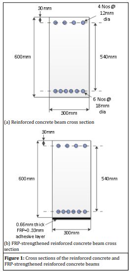
xX, i ' i,E V t x, i ' =min i= i ' n j=1 n π ¯ j e t1 p ¯ ji 1 a=1 A c a,x e,I + i= i ' n+1 j=1 k π ¯ j+n e t1 p ¯ jin 2 a=1 A c a,x e,I   + j=1 n π ¯ j e t1 p ¯ jn+1 1 a=1 A c a e,f + j=1 k π ¯ j+n e t1 p ¯ jk+1 2 a=1 A c a e,f + j=1 n+k π ¯ j e t a=1 A c a,j e,D 1 d t x, i ' d T,t                           (28) MathType@MTEF@5@5@+= feaahqart1ev3aaatCvAUfeBSjuyZL2yd9gzLbvyNv2CaerbuLwBLn hiov2DGi1BTfMBaeXatLxBI9gBaerbd9wDYLwzYbItLDharqqtubsr 4rNCHbGeaGqiVu0Je9sqqrpepC0xbbL8F4rqqrFfpeea0xe9Lq=Jc9 vqaqpepm0xbba9pwe9Q8fs0=yqaqpepae9pg0FirpepeKkFr0xfr=x fr=xb9adbiqaceGaciGaaiaabeqaamaabaabaaGcbaGaeyiaIiIaam iEaiabgIGiolaadIfacaGGSaGaamyAamaaCaaaleqabaGaai4jaaaa kiabgIGiolaadMgacaGGSaGaamyramaabmaabaGaamOvamaaBaaale aacaWG0baabeaakmaabmaabaGaamiEaiaacYcacaWGPbWaaWbaaSqa beaacaGGNaaaaaGccaGLOaGaayzkaaaacaGLOaGaayzkaaGaeyypa0 JaciyBaiaacMgacaGGUbWaamWaaqaabeqaamaaqahabaWaaabCaeaa cuaHapaCgaqeamaaDaaaleaacaWGQbaabaGaamyzaaaakmaabmaaba GaamiDaiabgkHiTiaaigdaaiaawIcacaGLPaaaceWGWbGbaebadaqh aaWcbaGaamOAaiaadMgaaeaacaaIXaaaaOWaaabCaeaacaWGJbWaa0 baaSqaaiaadggacaGGSaGaamiEaaqaaiaadwgacaGGSaGaamysaaaa aeaacaWGHbGaeyypa0JaaGymaaqaaiaadgeaa0GaeyyeIuoaaSqaai aadQgacqGH9aqpcaaIXaaabaGaamOBaaqdcqGHris5aaWcbaGaeyia IiIaamyAaiabg2da9iaadMgadaahaaadbeqaaiaacEcaaaWccqGHKj YOcaWGUbaabaaaniabggHiLdGccqGHRaWkdaaeWbqaamaaqahabaGa fqiWdaNbaebadaqhaaWcbaGaamOAaiabgUcaRiaad6gaaeaacaWGLb aaaOWaaeWaaeaacaWG0bGaeyOeI0IaaGymaaGaayjkaiaawMcaaiqa dchagaqeamaaDaaaleaacaWGQbGaamyAaiabgkHiTiaad6gaaeaaca aIYaaaaOWaaabCaeaacaWGJbWaa0baaSqaaiaadggacaGGSaGaamiE aaqaaiaadwgacaGGSaGaamysaaaaaeaacaWGHbGaeyypa0JaaGymaa qaaiaadgeaa0GaeyyeIuoaaSqaaiaadQgacqGH9aqpcaaIXaaabaGa am4AaaqdcqGHris5aaWcbaGaeyiaIiIaamyAaiabg2da9iaadMgada ahaaadbeqaaiaacEcaaaWccqGHLjYScaWGUbGaey4kaSIaaGymaaqa aaqdcqGHris5aaGcbaGaaeiiaiaabccacqGHRaWkdaaeWbqaaiqbec 8aWzaaraWaa0baaSqaaiaadQgaaeaacaWGLbaaaOWaaeWaaeaacaWG 0bGaeyOeI0IaaGymaaGaayjkaiaawMcaaiqadchagaqeamaaDaaale aacaWGQbGaamOBaiabgUcaRiaaigdaaeaacaaIXaaaaOWaaabCaeaa caWGJbWaa0baaSqaaiaadggaaeaacaWGLbGaaiilaiaadAgaaaaaba Gaamyyaiabg2da9iaaigdaaeaacaWGbbaaniabggHiLdaaleaacaWG QbGaeyypa0JaaGymaaqaaiaad6gaa0GaeyyeIuoakiabgUcaRmaaqa habaGafqiWdaNbaebadaqhaaWcbaGaamOAaiabgUcaRiaad6gaaeaa caWGLbaaaOWaaeWaaeaacaWG0bGaeyOeI0IaaGymaaGaayjkaiaawM caaiqadchagaqeamaaDaaaleaacaWGQbGaam4AaiabgUcaRiaaigda aeaacaaIYaaaaaqaaiaadQgacqGH9aqpcaaIXaaabaGaam4Aaaqdcq GHris5aOWaaabCaeaacaWGJbWaa0baaSqaaiaadggaaeaacaWGLbGa aiilaiaadAgaaaaabaGaamyyaiabg2da9iaaigdaaeaacaWGbbaani abggHiLdaakeaacqGHRaWkdaaeWbqaaiqbec8aWzaaraWaa0baaSqa aiaadQgaaeaacaWGLbaaaOWaaeWaaeaacaWG0baacaGLOaGaayzkaa WaaabCaeaacaWGJbWaa0baaSqaaiaadggacaGGSaGaamOAaaqaaiaa dwgacaGGSaGaamiraaaaaeaacaWGHbGaeyypa0JaaGymaaqaaiaadg eaa0GaeyyeIuoaaSqaaiaadQgacqGH9aqpcaaIXaaabaGaamOBaiab gUcaRiaadUgaa0GaeyyeIuoakmaabmaabaGaaGymaiabgkHiTmaala aabaGaamizamaaBaaaleaacaWG0baabeaakmaabmaabaGaamiEaiaa cYcacaWGPbWaaWbaaSqabeaacaGGNaaaaaGccaGLOaGaayzkaaaaba GaamizamaaBaaaleaacaWGubGaaiilaiaadshaaeqaaaaaaOGaayjk< aiaawMcaaaaacaGLBbGaayzxaaGaaeiiaiaabccacaqGGaGaaeiiai aabccacaqGGaGaaeiiaiaabccacaqGGaGaaeiiaiaabccacaqGGaGa aeiiaiaabccacaqGGaGaaeiiaiaabccacaqGGaGaaeiiaiaabccaca qGGaGaaeiiaiaabccacaqGGaGaaeiiaiaabccacaqGOaGaaeOmaiaa bIdacaqGPaaaaa@1F6A@

Example

The purpose of this example is to demonstrate the use of the proposed methodology to determine the optimal intervention strategies for a hypothetical bridge element, when the interventions could change the deterioration rate. FRP strengthening of reinforced concrete (RC) bridge girders was assumed to be one of the available intervention options. For illustrative purposes, representatives RC beam cross sections with and without FRP strengthening are provided in Figure 1.

With FRP strengthening, extended life spans can be expected for bridge structures, thus the life-span of the bridge was taken as 150 years. Calculations were carried out using the methodology presented in Section 2 for each year. The intervention strategy resulting in the minimum total cost up to 150 years was taken as the optimal intervention strategy. Also, the optimal intervention strategy was determined based on the simplified method presented in Section 3. Details of the example are given in the following sections.

CS definitions

Typically, the CSs of RC elements subjected to reinforcement corrosion are defined in terms of reinforcement section loss [15].Similarly, in the current study the CSs for the RC beam were defined based on the reinforcement section loss (Table 1). As the main deterioration of the FRP strengthened RC beam is the bond degradation, the CSs for the FRP strengthened RC beam were defined using the bond strength loss (Table 1). The CSs of the RC beam are denoted by CCS, while the CSs of FRP strengthened RC beam are denoted by FCS. The CSs of the FRP strengthened RC beam were set so that, the worst CS (i.e. FCS3) gives equal performance to the worst CS for the RC beam (i.e.CCS5). The structural failure probabilities corresponding to each CS are also given in Table 1 for both RC beam and FRP strengthened RC beam. As this example is only to illustrate the methodology, details of the structural failure probability calculations are not discussed

Deterioration matrices

The transition probabilities of the deterioration matrix for the RC beam without considering the failure probabilities are given in Table 2. Time interval is taken as one year. These transition probabilities could be easily obtained using a stochastic corrosion model [16-17]. As the corrosion initiation starts only in CCS2, there is no change in annual structural failure probability from CCS1 to CCS2. From CCS2 to CCS5, annual structural failure probabilities increase due to strength loss as a result of reinforcement section loss. In CCS5, RC girder will be considered as unsafe due to its excessively high structural failure probability.

The transition probabilities of the adjusted deterioration matrix (Equations 3 and 4) considering annual structural failure probabilities are given in Table 3.

The transition probabilities of the deterioration matrix for the FRP strengthened RC beam, without considering the structural failure probabilities are given in Table 4. These transition probabilities could be estimated using an appropriate bond-degradation model coupled with a bond-strength model [18-19].

The transition probabilities of the adjusted deterioration matrix (Equations3 and 4) considering annual structural failure probabilities are given in Table 5.

Intervention options

The transition probabilities for different intervention activities are shown in Table 6. In this table the rows correspond to the bridge girder condition before the intervention is applied (at the beginning of the time interval where the intervention will be carried out), whereas the columns refer to the CS in the year following the intervention. Four possible interventions: concrete cover repair (possible in CCSs 2 and 3), concrete spalling and reinforcement repair (possible in CCSs 2 to 5), replacement with a new concrete beam (possible in CCSs 2 to 5, FCS3 and the structural failure CS, i.e. CSF), and FRP strengthening (possible in CCSs 2 to 5) were considered.

The identified intervention options are possible for bridge girders either alone or in various combinations. The possible intervention combinations are normally determined by an expert engineer. In many practical situations, the number of intervention types and combinations will be limited to a finite set. For this example a hypothetical list of possible intervention sets and the CSs in which each intervention is permitted are given in Table 7. In total, 5 different intervention sets with 20 possible intervention strategies result from the list given in Table 7.

The costs corresponding to the CSs and intervention actions are given in Table 8. They are divided into owner and public costs. These costs are hypothetical. However efforts were made to keep the ratios of their magnitudes reasonable. For the owner, cover repair is very cheap ($15,000), compared to spalling and reinforcement repair ($30,000), FRP strengthening ($35,000) or replacement ($60,000). Spalling and reinforcement repair is still cheaper than FRP strengthening, owing to the high material costs of FRP (even though FRP strengthening will have lower construction costs). For the public, costs during the interventions depend on the intervention action. The public costs considered here include costs due to noise during construction, increased travel costs due to construction work, environmental costs, etc. When the bridge is close, traffic has to be detoured and assumed to translate into an additional public cost of $500 per day. If the bridge girder experiences structural failure, a relatively high cost ($400,000) is used to represent the possible injury and reconstruction costs.

The public costs due to normal operations of the bridge were assumed to be dependent on the CS, and taken as $20,000,$2 4,000,$28,000,$35,000, and $80,000 for CCS 1-5 respectively and $20,000,$24,000, and $60,000 for FCS1-3 respectively. The relatively high public costs associated with CCS5 and FCS3 are due to disturbances to the normal operations (e.g. restricted load limits, etc.) owing to the reduced safety of the bridge. A simple Microsoft Excel spreadsheet was setup to do the calculations.

Results

The calculation of the costs up to 150 years for all intervention strategies was easily done using the spreadsheet. The calculation effort for the simplified method was significantly less than that for the year-by-year life cycle cost analysis up to 150 years. Both methods are believed to be much easier than the existing methods, which may require time-consuming MC simulations.

The calculated costs over 150 years and annual costs using stead state properties are given in Table 9 for all of the intervention strategies. In order to compare the results, normalized total costs, i.e. normalized with respect to the minimum cost for each method, are given in the last two columns. These normalized costs of each strategy are also plotted in Figure 2. It is obvious that the results from the simplified method generally are in a good agreement with the calculated results over 150 years. The small differences were found to occur due to differences in cost calculations in the years before reaching the steady state. For some intervention strategies, it was also found that the steady state properties are not yet achieved during the 150 years. The optimal strategy selected from the cost minimization over 150 years was set 3, with interventions for CCS2, CCS4, FCS3, and CSF, while the optimal strategy selected using steady state properties was set 2 with interventions for CCS2, CCS4, and CSF. However, the difference between the costs obtained using steady state properties of these two intervention strategies was only 0.2%. Considering generally good agreement of two methods (Figure 2), the simplified method can be taken as a good approximate method to determine the optimal intervention strategy.

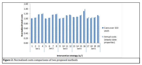
Table 1: CS description for reinforced concrete beams and FRP strengthened reinforced concrete beams


Condition state

Description

Failure probability

concrete beam

CCS1

as new, no corrosion

0.0001

CCS2

corrosion initiation, <2% thickness loss

0.0001

CCS3

moderate corrosion, <6% thickness loss

0.0002

CCS4

high corrosion, <12% thickness loss

0.0014

CCS5

severe corrosion, ≥12% thickness loss

0.0054

FRP strengthened concrete beam

FCS1

as new, loss in bond strength <10%

0.0000

FCS2

loss in bond strength 10-25%

0.0002

FCS3

loss in bond strength ≥25%

0.0034

Table 2: Transition probability matrix for reinforced concrete beam

Year (t)

Year ( t+1)


CS1

CS2

CS3

CS4

CS5

CS1

0.9180

0.0820

0.0000

0.0000

0.0000

CS2

0.0000

0.6200

0.3800

0.0000

0.0000

CS3

0.0000

0.0000

0.8410

0.1590

0.0000

CS4

0.0000

0.0000

0.0000

0.8940

0.1060

CS5

0.0000

0.0000

0.0000

0.0000

1.0000

Table 3: Adjusted transition probability matrix for reinforced concrete beams

Year (t)

Year ( t+1)


CS1

CS2

CS3

CS4

CS5

CSF

CS1

0.9179

0.0820

0.0000

0.0000

0.0000

0.0001

CS2

0.0000

0.6199

0.3800

0.0000

0.0000

0.0001

CS3

0.0000

0.0000

0.8408

0.1590

0.0000

0.0002

CS4

0.0000

0.0000

0.0000

0.8927

0.1059

0.0014

CS5

0.0000

0.0000

0.0000

0.0000

0.9946

0.0054

Table 4: Transition probability matrix for FRP strengthened beams

Year (t)

Year ( t+1)


FCS1

FCS2

FCS3

FCS1

0.9817

0.0183

0.0000

FCS2

0.0000

0.9878

0.0122

FCS3

0.0000

0.0000

1.0000

Table 5: Adjusted Transition probability matrix for FRP strengthened beams

Year (t)

Year ( t+1)


FCS1

FCS2

FCS3

CSF

FCS1

0.9817

0.0183

0.0000

0.0000

FCS2

0.0000

0.9877

0.0122

0.0001

FCS3

0.0000

0.0000

0.9992

0.0008

Table 6: Intervention options and their effectiveness

Intervention action

After the intervention

CS

CCS1

CCS2

CCS3

CCS4

CCS5

FCS1

FCS2

FCS3

Cover repair

CCS2

0.8500

0.0975

0.0525

0.0000

0.0000

0.0000

0.0000

0.0000

CCS3

0.5507

0.2662

0.1330

0.0501

0.0000

0.0000

0.0000

0.0000

Spalling and reinforcement repair

CCS2

0.9700

0.0300

0.0000

0.0000

0.0000

0.0000

0.0000

0.0000

CCS3

0.9600

0.0400

0.0000

0.0000

0.0000

0.0000

0.0000

0.0000

CCS4

0.9180

0.0820

0.0000

0.0000

0.0000

0.0000

0.0000

0.0000

CCS5

0.8000

0.1500

0.0500

0.0000

0.0000

0.0000

0.0000

0.0000

FRP strengthening

CCS2

0.0000

0.0000

0.0000

0.0000

0.0000

0.9817

0.0183

0.0000

CCS3

0.0000

0.0000

0.0000

0.0000

0.0000

0.9817

0.0183

0.0000

CCS4

0.0000

0.0000

0.0000

0.0000

0.0000

0.9817

0.0183

0.0000

CCS5

0.0000

0.0000

0.0000

0.0000

0.0000

0.9817

0.0183

0.0000

replacement with a concrete beam

CCS2

0.9180

0.0820

0.0000

0.0000

0.0000

0.0000

0.0000

0.0000

CCS3

0.9180

0.0820

0.0000

0.0000

0.0000

0.0000

0.0000

0.0000

CCS4

0.9180

0.0820

0.0000

0.0000

0.0000

0.0000

0.0000

0.0000

CCS5

0.9180

0.0820

0.0000

0.0000

0.0000

0.0000

0.0000

0.0000

FCS2

0.9180

0.0820

0.0000

0.0000

0.0000

0.0000

0.0000

0.0000

FCS3

0.9180

0.0820

0.0000

0.0000

0.0000

0.0000

0.0000

0.0000

CSF

0.9180

0.0820

0.0000

0.0000

0.0000

0.0000

0.0000

0.0000

Table 7: Possible intervention sets

Interventions set, x

Intervention action

Possible CSs, i'

1

Cover repair

CCS2, CCS3

Replacement

CCS4,CCS5,CSF

2

Cover repair

CCS2, CCS3

Spalling and reinforcement repair

CCS4,CCS5

Replacement

CSF

3

Cover repair

CCS2,CCS3

FRP strengthening

CCS4, CCS5

Replacement

FCS3, CSF

4

Spalling and reinforcement repair

CCS2, CCS3, CCS4, CCS5

Replacement

CSF

5

FRP Strengthening

CCS2, CCS3, CCS4, CCS5

Replacement

CSF, FCS3

Table 8: Bridge closure days and intervention costs

Intervention action

Applied CS

Number of bridge closure days

Costs (in thousands of dollars)

Owner

Public

Total

Cover repair

CCS2

2

15

2

17

CCS3

2

15

3

18

Spalling and reinforcement repair

CCS2

15

30

5

35

CCS3

15

30

5

35

CCS4

15

30

5

35

CCS5

15

30

5

35

FRP strengthening

CCS2

2

35

2

37

CCS3

2

35

2

37

CCS4

2

35

2

37

CCS5

2

35

2

37

Replacement (with a concrete beam)

CCS2

60

60

10

70

CCS3

60

60

10

70

CCS4

60

60

10

70

CCS5

60

60

10

70

FCS2

60

60

10

70

FCS3

60

60

10

70

CSF

90

300

400

700

Table 9: The calculated costs up to 150 years and annual costs from steady state properties

Intervention set, x

CSs of the interventions, i'

Total costs

Normalized total costs (Total cost/minimum total cost)

Costs up to 150 years

Annual costs (steady state properties)

Costs up to 150 years

Annual costs (steady state properties)

1

CCS2,CCS4,CSF

1086.54

22.57

1.012

1.011

CCS2,CCS5,CSF

1108.10

23.27

1.032

1.042

CCS3,CCS4,CSF

1256.04

26.33

1.169

1.179

CCS3,CCS5,CSF

1275.83

26.95

1.188

1.207

2

CCS2,CCS4,CSF

1076.49

22.32

1.002

1.000

CCS2,CCS5,CSF

1101.79

23.10

1.026

1.035

CCS3,CCS4,CSF

1244.19

26.06

1.158

1.167

CCS3,CCS5,CSF

1267.50

26.72

1.180

1.197

3

CCS2,CCS4,FCS3,CSF

1074.15

22.74

1.000

1.019

CCS2,CCS5,FCS3,CSF

1095.89

23.19

1.020

1.039

CCS3,CCS4,FCS3,CSF

1218.36

25.05

1.134

1.122

CCS3,CCS5,FCS3,CSF

1243.06

25.48

1.157

1.142

4

CCS2, CSF

1144.43

23.70

1.065

1.062

CCS3, CSF

1154.03

24.06

1.074

1.078

CCS4, CSF

1215.68

25.74

1.132

1.153

CCS5, CSF

1406.87

30.96

1.310

1.387

5

CCS2,FCS3, CSF

1083.25

23.51

1.008

1.053

CCS3,FCS3, CSF

1089.34

23.55

1.014

1.055

CCS4,FCS3,CSF

1119.97

23.78

1.043

1.065

CCS5,FCS3,CSF

1225.74

24.77

1.141

1.110

Conclusions

This paper presents a methodology for evaluating the lifecycle impacts of intervention strategies for infrastructure such as bridges, which considers the possible changing deterioration rates due to interventions during the service life. The methodology was developed based on the Markovian approach commonly used in existing bridge management systems. The safety of the structure was also considered by introducing an additional condition state. Based on the steady state properties, a simplified method was proposed to determine the optimal intervention strategies.

The proposed methodology is demonstrated for a hypothetical concrete bridge girder, where one of the intervention options is FRP strengthening. Several intervention options resulting in 20 intervention strategies were compared. The optimal strategy was selected based on minimum total life-cycle cost up to 150 years as well as based on minimum annual costs determined using steady state probabilities.

The results showed that the proposed method can be effectively used to evaluate intervention strategies that result in deterioration rate changes, also in order to determine the optimal intervention strategies. Results from the simplified model show a good agreement with the results from the year-by-year life-cycle cost analysis. However, some discrepancies occurred due to steady state not yet being reached during the 150 year analysis period and/or due to differences in costs in the early years (before the steady state is reached). Nevertheless, the proposed methodology is seen to provide an efficient means of considering the effects of changing deterioration rates in evaluating the life-cycle impacts of intervention strategies.

References

  1. Scherer WT, Glagola DM. Markovian models for bridge maintenance management. Journal of Transportation Engineering. 1994;120(1):37-51.
  2. Roelfstra G. Modeled' evolution de l'etat des ponts-routes enbeton. These n°2310 – Grade de Docteurès Sciences Techniques, Doctoral Dissertation, ÉcolePolytechniqueFédéral de Lausanne. Switzerland (in French), 2001.
  3. Orcesi A,Cremona C. Optimization of maintenance strategies for the management of the national bridge stock in France. Journal of Bridge Engineering, ASCE. 2011;16(1):44–52.
  4. Almeida J, Teixeira P,Delgado R. Life cycle cost optimisation in highway concrete bridges management. Structure and Infrastructure Engineering. 2013;1-14.
  5. Walbridge S, Fernando D, Adey BT. Cost-benefit analysis of alternative corrosion management strategies for a steel roadway bridge.Journal of Bridge Engineering,ASCE. 2013;18(4):318-327.
  6. Fernando D, Mirazei Z, Adey BT, Ellis RM. The application of benefit hierarchy to determine the optimal intervention strategies for bridges. Transportation Research Board 91st Annual Meeting. 2012:22-26, Washington D.C.
  7. Thompson PD, Small EP, Johnson M, Marshall AR. The Pontis bridge management system. Structural Engineering International, IABSE. 1998;8:303-308.
  8. Pontis. Version 4.0 Technical Manual Report. USA: FHWA, US Department of Transportation. USA, 2001.
  9. KUBA. KUBA-MS-Ticino-user's manual, release 3.0., F.D.o. Highways, Bern, Switzerland, 2005.
  10. Jiang Y, Sinha KC. Bridge service life prediction model using markov chain. Transportation Research Record. 1989;1223:24-30.
  11. Toutanji H, Gomez W. Durability characteristics of concrete beams externally bonded with FRP composite sheets. Cement and Concrete Composites. 1997;19:351-358.
  12. Karbhari VM, Chin JW, Hunston D, Benmokrane B, Juska T, Morgan R, Lesko JJ, Sorathia U, Reynaud D. Durability gap analysis for fiber-reinforced polymer composites in civil infrastructure. Journal of Composites for Construction, ASCE. 2003;7 (3):238-247.
  13. Robelin CA, Madanat S. History-dependent bridge deck maintenance and replacement optimization with Markov decision processes, Journal of Infrastructure Systems, ASCE. 2007;13(3):195-201.
  14. Ching WK, Huang X, Ng MK, Siu TK. Markov chains: models, algorithms and applications.International series in operations research & management science. Springer Science Business Media. 2013;189: New York, USA.
  15. Pontis. Pontis Bridge Inspection Manual. M.D.o. Transportation, Michigan, USA, 2007.
  16. Pedersen C, Thoft-Christensen P. Reliability analysis of prestressed concrete beams with corroded tendons.Instituttet for Bygningsteknik, Aalborg Universitetscenter, 1993.
  17. Vu KAT, Stewart MG. Structural reliability of concrete bridges including improved chloride-induced corrosion models. Structural Safety. 2000;22:313-333.
  18. Ouyang Z, Wan B. Modeling of moisture diffusion in FRP strengthened concrete specimens. Journal of Composites for Construction, ASCE. 2008;12(4):425-434.
  19. Tuakta C, Büyüköztürk O. Conceptual model for prediction of FRP-concrete bond strength under moisture cycles. Journal of Composites for Construction, ASCE. 2011;15(5):743-756.